Clustering

Clustering algorithms group data into clusters based on similarity, without predefined labels. This is the second major branch of classical unsupervised machine learning, alongside the dimensionality reduction methods we have just covered.

These notes cover:

• clustering versus supervised classification, and what clustering is good for

• the landscape of clustering algorithms, and their trade-offs

• K-means clustering — the algorithm, and its failure modes

• how to choose the number of clusters (inertia and the elbow method, the silhouette score)

• DBSCAN

• Gaussian Mixture Models

Clustering vs. supervised classification

The contrast with supervised classification is the place to start. In classification we already have labels, and we are predicting them based on known outcomes. In clustering we have no labels a priori, and we are trying to discover the inherent patterns and relationships in the data.

import numpy as np
import matplotlib.pyplot as plt
from sklearn.datasets import load_iris

iris = load_iris()
X = iris.data[:, 2:4]      # petal length, petal width
y = iris.target

fig, (ax1, ax2) = plt.subplots(1, 2, figsize=(12, 5))

# Supervised: we know the labels, and color by them.
for k, name in enumerate(iris.target_names):
    ax1.scatter(X[y == k, 0], X[y == k, 1], label=name, edgecolor="k", s=40, alpha=0.8)
ax1.set_xlabel("petal length (cm)")
ax1.set_ylabel("petal width (cm)")
ax1.set_title("Supervised classification: labels are known")
ax1.legend()
ax1.grid(alpha=0.3)

# Unsupervised: this is all a clustering algorithm ever sees.
ax2.scatter(X[:, 0], X[:, 1], c="gray", edgecolor="k", s=40, alpha=0.8)
ax2.set_xlabel("petal length (cm)")
ax2.set_ylabel("petal width (cm)")
ax2.set_title("Clustering: no labels — find the groups yourself")
ax2.grid(alpha=0.3)

plt.tight_layout()
plt.show()

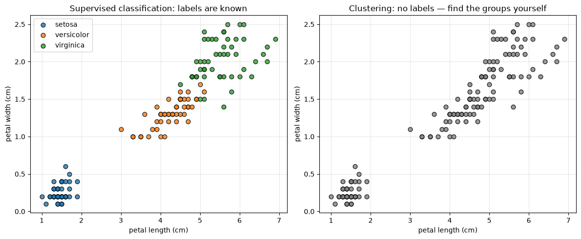
Look at the right-hand panel — that is all a clustering algorithm gets. The bottom-left group is obviously separate, and any method will find it. But knowing how to split the other two would be much harder without the labels: they run together. That is the challenge of clustering in a nutshell.

Clustering is useful for:

• Data analysis — discovering structure you didn’t know was there

• Dimensionality reduction

• Anomaly detection — if we have some well-defined clusters and then see points lying well outside of them, that suggests anomalous or unusual samples worth analyzing further. In climate and environmental science this could be an unusual soil or water sample, an unusual weather pattern, or an instrument that has developed a fault and is reporting something not typically represented in the data set.

There are many different clustering algorithms

Different algorithms are built on different principles, and they behave very differently depending on how your data is actually distributed. The figure below applies four common methods to five differently-shaped data sets.

from sklearn import cluster, mixture
from sklearn.datasets import make_blobs, make_circles, make_moons
from sklearn.preprocessing import StandardScaler
import time
import warnings

rng = np.random.default_rng(0)
n = 500

# Five data sets with deliberately different structure.
circles = make_circles(n_samples=n, factor=0.5, noise=0.05, random_state=0)[0]
moons = make_moons(n_samples=n, noise=0.05, random_state=0)[0]
blobs = make_blobs(n_samples=n, random_state=8)[0]
# Anisotropic (stretched, ellipsoidal) blobs
Xa = make_blobs(n_samples=n, random_state=170)[0]
aniso = Xa @ [[0.6, -0.6], [-0.4, 0.8]]
# Blobs with very different variances
varied = make_blobs(n_samples=n, cluster_std=[1.0, 2.5, 0.5], random_state=170)[0]

datasets = [("circles", circles, 2), ("moons", moons, 2), ("varied", varied, 3),
            ("aniso", aniso, 3), ("blobs", blobs, 3)]

algos = ["K-Means", "MiniBatch K-Means", "DBSCAN", "Gaussian Mixture"]

fig, axes = plt.subplots(len(datasets), len(algos), figsize=(13, 15))

for row, (dname, Xd, k) in enumerate(datasets):
    Xd = StandardScaler().fit_transform(Xd)
    models = [
        cluster.KMeans(n_clusters=k, n_init=10, random_state=0),
        cluster.MiniBatchKMeans(n_clusters=k, n_init=10, random_state=0),
        cluster.DBSCAN(eps=0.3),
        mixture.GaussianMixture(n_components=k, covariance_type="full", random_state=0),
    ]
    for col, (aname, model) in enumerate(zip(algos, models)):
        ax = axes[row, col]
        t0 = time.time()
        with warnings.catch_warnings():
            warnings.simplefilter("ignore")
            model.fit(Xd)
        elapsed = time.time() - t0
        pred = model.predict(Xd) if hasattr(model, "predict") else model.labels_

        ax.scatter(Xd[:, 0], Xd[:, 1], c=pred, cmap="tab10", s=8)
        ax.set_xticks([]); ax.set_yticks([])
        if row == 0:
            ax.set_title(aname, size=11)
        if col == 0:
            ax.set_ylabel(dname, size=11)
        # Runtime matters as much as accuracy — note it in the corner.
        ax.text(0.99, 0.01, f"{elapsed*1000:.0f} ms", transform=ax.transAxes,
                size=9, ha="right", color="dimgray")

plt.tight_layout()
plt.show()

Reading across the rows, some methods do much better than others depending on the shape of the clusters and how they sit relative to one another. K-means handles the well-separated blobs beautifully and the circles and moons terribly. DBSCAN handles the moons and circles — the non-convex shapes — but is thrown by varied, where cluster densities differ. The Gaussian Mixture Model handles aniso, the stretched clusters, far better than K-means does.

Also note the runtimes in the corner of each panel. This is a real trade-off: a method like OPTICS works well across many of these data sets but is one of the most computationally expensive available. Depending on how your data points are distributed, how much time you have, and how large your data set is, some methods will be more usable than others.

We’ll cover K-means, DBSCAN, and Gaussian Mixture Models below, but there are many more. It is worth exploring the scikit-learn clustering documentation for whatever data set you are actually trying to cluster.

K-means clustering

K-means is one of the classic, older clustering methods, and it has been around a very long time.

The assumption you must make as the user is how many clusters are present in the data to begin with. The number of clusters, \(K\), is a hyperparameter of the algorithm — the algorithm cannot tell you it.

Each sample \(\mathbf{x}_i\) will be assigned one (and only one) cluster; samples cannot belong to several clusters at once. We write \(C(i)\) for the cluster number of the \(i\)th observation. Our dissimilarity measure is the Euclidean distance — effectively the vector distance between two points in feature space.

K-means minimizes the within-cluster point scatter:

\[W(C) = \sum_{k=1}^{K} \sum_{C(i)=k} \lVert \mathbf{x}_i - \mathbf{m}_k \rVert^2\]

where \(\mathbf{m}_k\) is the mean (the centroid) of cluster \(k\).

The algorithm

1. Randomly initialize \(K\) initial centroids.

2. Assign each observation \(\mathbf{x}_i\) to its nearest centroid.

3. For a given cluster assignment \(C\), compute the cluster means:

   \[\mathbf{m}_k = \frac{1}{N_k}\sum_{C(i)=k} \mathbf{x}_i\]

4. For the current set of cluster means, reassign each observation:

   \[C(i) = \arg\min_{1 \le k \le K} \lVert \mathbf{x}_i - \mathbf{m}_k \rVert^2\]

5. Iterate steps 3 and 4 until convergence — until the centroids stop moving.

from sklearn.cluster import KMeans

# Five clusters, some more spread out than others. We keep the true labels y5
# only to score the algorithms below — K-means itself never sees them.
X5, y5 = make_blobs(n_samples=800, centers=[[-2.5, 3], [0.5, 4.5], [-1.5, 0],
                                            [3, 1.5], [4, 3.5]],
                    cluster_std=[0.5, 0.4, 0.9, 0.35, 0.4], random_state=7)

def plot_state(ax, X, centroids, title, show_boundaries=True):
    if show_boundaries:
        # Color the plane by which centroid is nearest — the decision boundaries.
        h = 0.03
        xx, yy = np.meshgrid(np.arange(X[:, 0].min()-1, X[:, 0].max()+1, h),
                             np.arange(X[:, 1].min()-1, X[:, 1].max()+1, h))
        grid = np.c_[xx.ravel(), yy.ravel()]
        d = ((grid[:, None, :] - centroids[None, :, :]) ** 2).sum(-1)
        ax.contourf(xx, yy, d.argmin(1).reshape(xx.shape), alpha=0.25, cmap="tab10")
    ax.plot(X[:, 0], X[:, 1], "k.", markersize=2)
    ax.scatter(centroids[:, 0], centroids[:, 1], marker="X", s=200,
               c="red", edgecolor="k", linewidth=1.5, zorder=10)
    ax.set_title(title, size=11)
    ax.set_xticks([]); ax.set_yticks([])

# Step through the first few iterations by capping max_iter.
fig, axes = plt.subplots(2, 3, figsize=(14, 8))
rng = np.random.default_rng(2)
init = X5[rng.choice(len(X5), 5, replace=False)]   # random initial centroids

plot_state(axes[0, 0], X5, init, "1. Randomly initialize 5 centroids", show_boundaries=False)
plot_state(axes[0, 1], X5, init, "2. Assign each point to its nearest centroid")

for ax, iters in zip([axes[0, 2], axes[1, 0], axes[1, 1]], [1, 2, 3]):
    km = KMeans(n_clusters=5, init=init, n_init=1, max_iter=iters, random_state=0).fit(X5)
    plot_state(ax, X5, km.cluster_centers_, f"3-4. After {iters} update(s)")

km_final = KMeans(n_clusters=5, init=init, n_init=1, random_state=0).fit(X5)
plot_state(axes[1, 2], X5, km_final.cluster_centers_, "5. Converged")

plt.tight_layout()
plt.show()

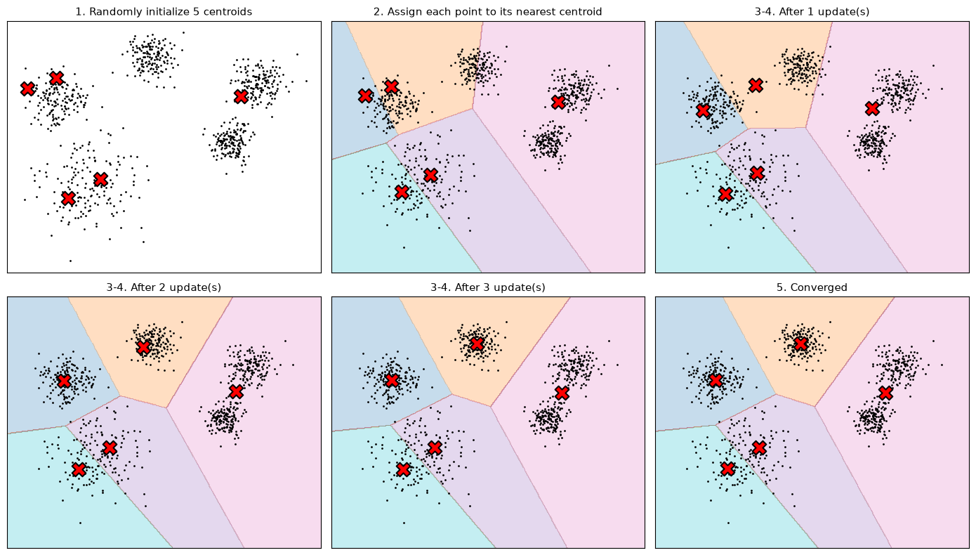
The shaded regions are the decision boundaries: every point in a shaded region is nearer to that region’s centroid than to any other. Watch the centroids march toward the centers of the clusters as the iterations proceed. Each update recomputes the centroid as the mean of the points currently assigned to it, which pulls it toward the cluster’s true center, which changes the assignments, and so on until nothing moves. For a data set like this — well-separated, roughly round, comparable densities — K-means does a good job.

K-means does not have a unique solution

Because the centroids are randomly initialized, running K-means more than once will not give exactly the same solution. Iteratively minimizing the inertia — scikit-learn’s name for exactly the \(W(C)\) we wrote down above, the sum of squared distances from every point to its assigned centroid — does not guarantee a unique answer. The algorithm can settle into different local minima depending on where it started.

from sklearn.metrics import adjusted_rand_score

fig, axes = plt.subplots(1, 2, figsize=(12, 5))

for ax, seed in zip(axes, [3, 0]):
    rng = np.random.default_rng(seed)
    init = X5[rng.choice(len(X5), 5, replace=False)]
    km = KMeans(n_clusters=5, init=init, n_init=1, random_state=0).fit(X5)
    plot_state(ax, X5, km.cluster_centers_,
               f"Random start {seed} — inertia = {km.inertia_:.0f}")
    # y5 holds the true cluster each point came from. The Adjusted Rand Index
    # scores the clustering against it: 1.0 is a perfect match, 0.0 is random.
    print(f"random start {seed}: inertia = {km.inertia_:7.1f}, "
          f"agreement with true clusters (ARI) = {adjusted_rand_score(y5, km.labels_):.3f}")

plt.tight_layout()
plt.show()

random start 3: inertia =   438.2, agreement with true clusters (ARI) = 0.988
random start 0: inertia =  1250.0, agreement with true clusters (ARI) = 0.718

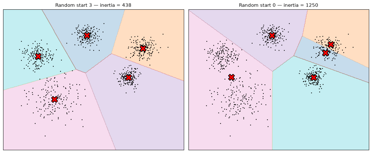
Two different initializations, two genuinely different answers — and one is much worse than the other. The good run finds the five real clusters almost exactly (ARI 0.99). The bad run gets stuck in a local minimum with nearly three times the inertia: it has balanced a centroid between two real clusters and then split a single real cluster in two to compensate, which is why it only scores 0.72.

Both are legitimate stopping points for the algorithm — neither can improve by moving a single centroid. Nothing about the second run is a bug; it is just where that particular random start happened to lead.

In practice scikit-learn guards against this by running the algorithm several times from different random initializations and keeping the best result — that is what the n_init parameter controls. Above we set n_init=1 deliberately, to expose the underlying behavior.

How to choose the number of clusters?

The other challenge is that we have to know \(K\) a priori, and often we don’t. If we are looking at some environmental variables we have measured, we may have no idea how many classes are actually represented in the data.

fig, axes = plt.subplots(1, 2, figsize=(12, 5))
for ax, k in zip(axes, [3, 8]):
    km = KMeans(n_clusters=k, n_init=10, random_state=0).fit(X5)
    plot_state(ax, X5, km.cluster_centers_, f"K = {k}")
plt.tight_layout()
plt.show()

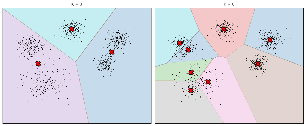
Both of these produce an answer. Neither tells you it is the wrong one. So how do we choose?

The elbow method

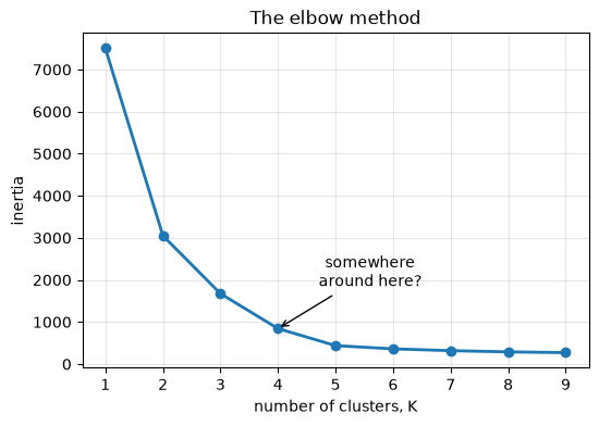
Plot the inertia — the sum of squared distances from every point to its assigned centroid — against the number of clusters. Inertia always decreases as \(K\) grows (with \(K\) equal to the number of samples it reaches zero), so we can’t just minimize it. Instead we look for the elbow: the point where the curve stops dropping steeply and starts decreasing much more slowly.

ks = list(range(1, 10))
inertias = [KMeans(n_clusters=k, n_init=10, random_state=0).fit(X5).inertia_ for k in ks]

plt.figure(figsize=(6, 4))
plt.plot(ks, inertias, "o-", lw=2)
plt.xlabel("number of clusters, K")
plt.ylabel("inertia")
plt.annotate("somewhere\naround here?", xy=(4, inertias[3]), xytext=(5.6, inertias[3] * 2.2),
             arrowprops=dict(arrowstyle="->"), ha="center")
plt.title("The elbow method")
plt.grid(alpha=0.3)
plt.show()

# The bend is easier to judge from how much each extra cluster buys you.
print("  K :  inertia : drop from K-1")
for i, (k, v) in enumerate(zip(ks, inertias)):
    drop = f"{inertias[i-1] - v:8.0f}" if i else "       -"
    print(f"  {k} : {v:8.0f} : {drop}")

  K :  inertia : drop from K-1
  1 :     7504 :        -
  2 :     3051 :     4453
  3 :     1674 :     1377
  4 :      843 :      831
  5 :      438 :      405
  6 :      361 :       77
  7 :      318 :       43
  8 :      289 :       29
  9 :      271 :       18

The inertia has an elbow, but it is not always enough to objectively choose \(K\).

Look at the printed drops rather than the picture. Going from 4 to 5 clusters still buys a substantial reduction in inertia (~405), and only after \(K=5\) does the curve really flatten (~77). So the bend is arguably at 5 — which is what we built. But the bend is gradual, and that is the problem: reading this curve by eye you could justify 4 or 5, and a standard automated knee-finding rule applied to it actually returns 3. The elbow gives you a range, not an answer.

This is worse when clusters have different densities, as they do here: some are tightly packed and some are spread out, and inertia is dominated by the spread-out ones, which keep rewarding extra splits regardless of the true cluster count.

The silhouette score

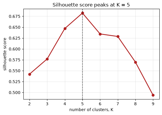
An alternative is the silhouette score, which balances the distance to a point’s own cluster against its distance to the nearest other cluster. For a single sample:

\[s = \frac{b - a}{\max(a, b)}\]

where

• \(a\) = the mean distance to the other instances in the same cluster (how tight its own cluster is around it)

• \(b\) = the mean nearest-cluster distance — the mean distance to the instances of the closest cluster that the sample is not part of

The score ranges from \(-1\) to \(+1\). A value near \(+1\) means the sample is comfortably inside its own cluster and far from the next one; near \(0\) means it sits on a boundary; negative means it has probably been assigned to the wrong cluster. We average this over all samples.

from sklearn.metrics import silhouette_score

ks = range(2, 10)
sil = [silhouette_score(X5, KMeans(n_clusters=k, n_init=10, random_state=0).fit_predict(X5))
       for k in ks]

plt.figure(figsize=(6, 4))
plt.plot(ks, sil, "o-", lw=2, color="firebrick")
best = ks[int(np.argmax(sil))]
plt.axvline(best, ls=":", c="k")
plt.xlabel("number of clusters, K")
plt.ylabel("silhouette score")
plt.title(f"Silhouette score peaks at K = {best}")
plt.grid(alpha=0.3)
plt.show()

print("silhouette score by K:")
for k, s in zip(ks, sil):
    print(f"  K = {k}: {s:.3f}")

silhouette score by K:
  K = 2: 0.542
  K = 3: 0.577
  K = 4: 0.647
  K = 5: 0.682
  K = 6: 0.634
  K = 7: 0.629
  K = 8: 0.570
  K = 9: 0.494

The silhouette score peaks unambiguously at 5 — the number of clusters we actually built into the data — and by a clear margin over its neighbors (0.682 against 0.647 at \(K=4\)). Where the inertia curve gave us a soft bend we had to squint at, the silhouette score gives us a maximum we can just read off. That is what makes it the more objective of the two.

It is not infallible — it is still a heuristic, and it has its own bias toward convex, well-separated clusters. But when the elbow is ambiguous, the silhouette score is usually the better guide.

Advantages and disadvantages of K-means

K-means is fast and scalable, and it is a very simple algorithm to use. But it can struggle with clusters of varying sizes, varying densities, and non-spherical shapes.

Variants such as accelerated K-means and mini-batch K-means improve on efficiency, speed, and scalability, but they don’t change the underlying assumptions.

# Ellipsoidal (anisotropic) clusters — K-means' classic failure case.
Xa_raw, ya_raw = make_blobs(n_samples=500, random_state=170)
X_aniso = Xa_raw @ [[0.6, -0.6], [-0.4, 0.8]]

km_a = KMeans(n_clusters=3, n_init=10, random_state=0).fit(X_aniso)

plt.figure(figsize=(6, 5))
plt.scatter(X_aniso[:, 0], X_aniso[:, 1], c=km_a.labels_, cmap="tab10", s=12)
plt.scatter(km_a.cluster_centers_[:, 0], km_a.cluster_centers_[:, 1],
            marker="X", s=250, c="red", edgecolor="k", linewidth=1.5, zorder=10)
plt.title(f"K-means on stretched clusters (inertia = {km_a.inertia_:.0f})")
plt.xticks([]); plt.yticks([])
plt.show()

print(f"agreement with the true clusters (ARI) = "
      f"{adjusted_rand_score(ya_raw, km_a.labels_):.3f}")

agreement with the true clusters (ARI) = 0.555

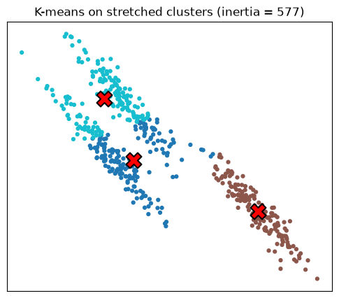
These clusters are stretched and skewed rather than round. K-means slices across them, placing centroids between the true clusters, because it is minimizing squared distance to a center and has no concept of a cluster having a direction.

Note what the ARI is telling us. K-means converged happily and reported a perfectly respectable inertia — by its own objective, nothing went wrong. But scored against the clusters that are actually there, it only manages about 0.56. A low inertia does not mean a good clustering; it only means the algorithm did well at the thing it was optimizing, which is not the same thing.

K-means works best when clusters have similar densities, are reasonably well separated, and are roughly spherical — the blobs case in the comparison figure above. Once you have more complex shapes or differing densities, you need something else.

DBSCAN

DBSCAN — Density-Based Spatial Clustering of Applications with Noise — takes a different approach. It finds core samples of high density and then expands clusters outward from them. Where K-means is top-down (start with \(K\) centers, assign everything), DBSCAN is bottom-up: find the dense regions of the data set, then grow them by adding neighboring points.

DBSCAN works well when the data contains clusters of similar density, separated by regions of lower density.

Its key hyperparameter is eps: the maximum distance between two samples for one to be considered a neighbor of the other. This is the most important parameter to get right for DBSCAN, and it makes a large difference.

from sklearn.cluster import DBSCAN

X_moons, _ = make_moons(n_samples=1000, noise=0.06, random_state=42)

fig, axes = plt.subplots(1, 3, figsize=(15, 4.5))

# K-means for reference: it cannot handle non-convex shapes.
km_m = KMeans(n_clusters=2, n_init=10, random_state=0).fit(X_moons)
axes[0].scatter(X_moons[:, 0], X_moons[:, 1], c=km_m.labels_, cmap="tab10", s=8)
axes[0].set_title("K-means (K=2): splits the moons the wrong way")

for ax, eps in zip(axes[1:], [0.05, 0.2]):
    db = DBSCAN(eps=eps).fit(X_moons)
    n_clusters = len(set(db.labels_)) - (1 if -1 in db.labels_ else 0)
    n_noise = (db.labels_ == -1).sum()
    ax.scatter(X_moons[:, 0], X_moons[:, 1], c=db.labels_, cmap="tab10", s=8)
    ax.set_title(f"DBSCAN, eps = {eps}\n{n_clusters} clusters, {n_noise} points marked noise")

for ax in axes:
    ax.set_xticks([]); ax.set_yticks([])
plt.tight_layout()
plt.show()

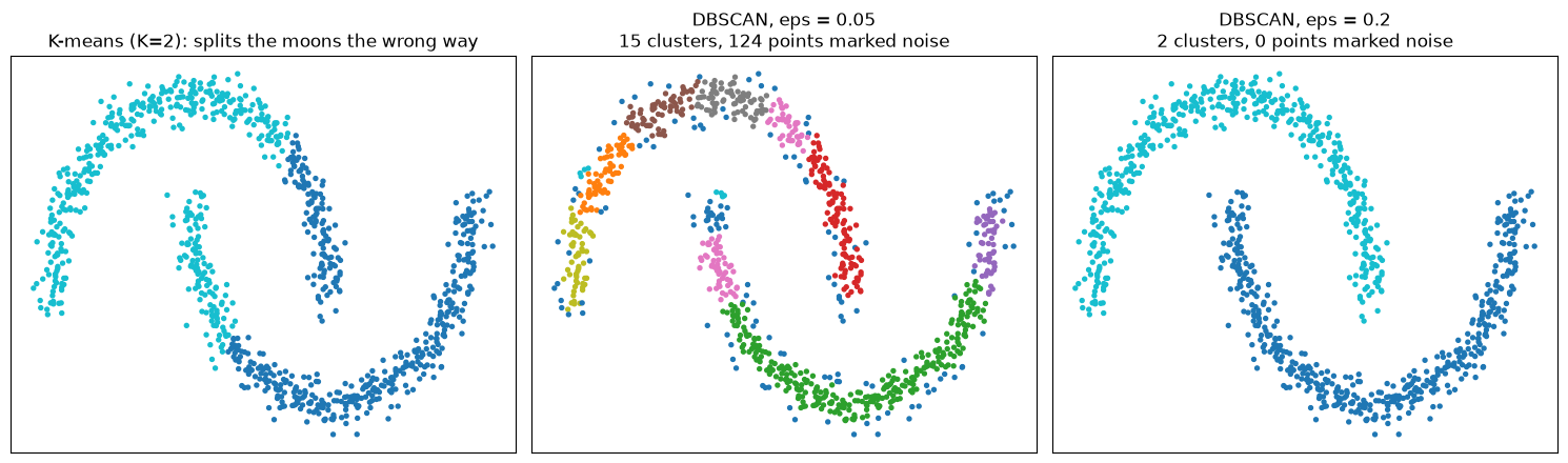
In contrast to K-means, DBSCAN does a good job of capturing these u-shaped clusters, which K-means simply cannot — a straight decision boundary can’t wrap around a crescent.

But look at the effect of eps. Set too low (middle panel), DBSCAN tries to break each moon into many separate sub-clusters, finding far more clusters than are really there. Set appropriately (right panel), it identifies the two real clusters cleanly. Setting these hyperparameters correctly makes a big difference to how well the algorithm performs.

DBSCAN is also robust to outliers, more so than K-means. It is allowed to label a point as belonging to no cluster at all — those are the “noise” points counted above. K-means, by contrast, always uses every point in the data set, because it recalculates centroids as means; a few distant outliers can drag a centroid away and throw off the whole clustering. DBSCAN just excludes a point that is too far from any cluster and where the density is too low. If your data set has outliers, DBSCAN may be preferable.

Gaussian Mixture Models

A Gaussian Mixture Model (GMM) is a probabilistic model that assumes all data points are generated from a mixture of a finite number of Gaussian distributions with unknown parameters.

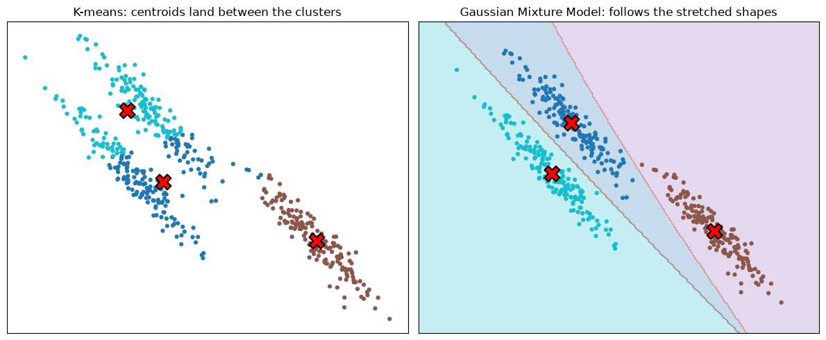
You can think of a GMM as a generalization of K-means that also includes information about the covariance structure of the data. K-means only knows where a cluster’s center is. A GMM also knows its shape and orientation — so a cluster that has been stretched and skewed relative to a typical Gaussian is still something it can represent.

In practice, that means a GMM handles the ellipsoidal clusters that defeated K-means.

from sklearn.mixture import GaussianMixture

gmm = GaussianMixture(n_components=3, covariance_type="full", random_state=42).fit(X_aniso)
labels_gmm = gmm.predict(X_aniso)

fig, (ax1, ax2) = plt.subplots(1, 2, figsize=(12, 5))

ax1.scatter(X_aniso[:, 0], X_aniso[:, 1], c=km_a.labels_, cmap="tab10", s=12)
ax1.scatter(km_a.cluster_centers_[:, 0], km_a.cluster_centers_[:, 1],
            marker="X", s=250, c="red", edgecolor="k", linewidth=1.5, zorder=10)
ax1.set_title("K-means: centroids land between the clusters")

# Shade the GMM's decision boundaries so the comparison is like-for-like.
h = 0.05
xx, yy = np.meshgrid(np.arange(X_aniso[:, 0].min()-1, X_aniso[:, 0].max()+1, h),
                     np.arange(X_aniso[:, 1].min()-1, X_aniso[:, 1].max()+1, h))
Z = gmm.predict(np.c_[xx.ravel(), yy.ravel()]).reshape(xx.shape)
ax2.contourf(xx, yy, Z, alpha=0.25, cmap="tab10")
ax2.scatter(X_aniso[:, 0], X_aniso[:, 1], c=labels_gmm, cmap="tab10", s=12)
ax2.scatter(gmm.means_[:, 0], gmm.means_[:, 1], marker="X", s=250,
            c="red", edgecolor="k", linewidth=1.5, zorder=10)
ax2.set_title("Gaussian Mixture Model: follows the stretched shapes")

for ax in (ax1, ax2):
    ax.set_xticks([]); ax.set_yticks([])
plt.tight_layout()
plt.show()

print("on the same stretched clusters:")
print(f"  K-means          ARI = {adjusted_rand_score(ya_raw, km_a.labels_):.3f}")
print(f"  Gaussian Mixture ARI = {adjusted_rand_score(ya_raw, labels_gmm):.3f}")

on the same stretched clusters:
  K-means          ARI = 0.555
  Gaussian Mixture ARI = 1.000

This is the same data set that K-means struggled with. Where K-means put its centroids between the ellipsoidal clusters and scored about 0.56, the GMM recovers the true clusters exactly — because it can model the covariance, the stretch and tilt, of each one.

A GMM is also probabilistic: rather than a hard assignment, predict_proba gives you the probability that each point belongs to each cluster, which is useful when you want to express uncertainty about boundary cases. (On this particular data set the clusters are well enough separated that almost every point is assigned with near-total confidence, so there is little uncertainty to look at — but the machinery is there when your clusters do overlap.)

As with everything here, it depends on your specific data: how the points are laid out in your clusters, and what shape those clusters are.

Summary

Method	Key hyperparameter	Good at	Struggles with
K-means	n_clusters	Fast, scalable, round well-separated clusters of similar density	Varying sizes/densities, non-spherical shapes, outliers; no unique solution
DBSCAN	eps	Non-convex shapes; robust to outliers; finds its own cluster count	Clusters of differing density; sensitive to eps
Gaussian Mixture	n_components	Ellipsoidal clusters; covariance structure; probabilistic assignments	Still assumes Gaussian components; need to choose the component count

There are a number of different clustering methods beyond these three, built on different principles and suited to different data. Explore the scikit-learn documentation for the data set you are working with.

Recall too that clustering is often used in combination with dimensionality reduction: first find a transformation into a space where the classes separate more easily, then cluster in that space. Together they give us unsupervised classification, without ever starting from labeled data.