Decision Trees and Random Forests (Wildfire cause prediction)

In this lesson, we will learn about decision trees and random forests and how they can be used for supervised machine learning tasks such as classification. A decision tree is an algorithm that can be used to determine how to classify or predict a target by making sequential decisions about the values of different features associated with a sample. Random forests use the ensemble vote of many decision trees to classify or predict a value.

We will use the data set from the paper “Inference of Wildfire Causes From Their Physical, Biological, Social and Management Attributes” by Pourmohamad et al., Earth’s Future, 2025. In this paper, they explored whether its possible to determine the cause of a wildfire (in cases where the cause is unknown) based on data from other wildfires where the cause was known.

References:

[1] Pourmohamad, Y., Abatzoglou, J. T., Fleishman, E., Short, K. C., Shuman, J., AghaKouchak, A., et al. (2025). Inference of wildfire causes from their physical, biological, social and management attributes. Earth’s Future, 13, e2024EF005187. https://doi.org/10.1029/2024EF005187

[2] Pourmohamad, Y., Abatzoglou, J. T., Belval, E. J., Fleishman, E., Short, K., Reeves, M. C., Nauslar, N., Higuera, P. E., Henderson, E., Ball, S., AghaKouchak, A., Prestemon, J. P., Olszewski, J., and Sadegh, M.: Physical, social, and biological attributes for improved understanding and prediction of wildfires: FPA FOD-Attributes dataset, Earth Syst. Sci. Data, 16, 3045–3060, https://doi.org/10.5194/essd-16-3045-2024, 2024.

[3] Pourmohamad, Y. (2024). Inference of Wildfire Causes from Their Physical, Biological, Social and Management Attributes (0.1). Zenodo. https://doi.org/10.5281/zenodo.11510677

import pandas as pd
import seaborn as sns
import os
import numpy as np`

Load in the data set

The data set can be downloaded from “https://zenodo.org/records/11510677”.

!wget "https://zenodo.org/records/11510677/files/FPA_FOD_west_cleaned.csv" data/.

--2025-09-04 14:38:31--  https://zenodo.org/records/11510677/files/FPA_FOD_west_cleaned.csv
Resolving zenodo.org (zenodo.org)... 188.185.43.25, 188.185.45.92, 188.185.48.194
Connecting to zenodo.org (zenodo.org)|188.185.43.25|:443... connected.
HTTP request sent, awaiting response... 200 OK
Length: 139402360 (133M) [text/plain]
Saving to: ‘FPA_FOD_west_cleaned.csv.9’

FPA_FOD_west_cleane 100%[===================>] 132.94M  8.12MB/s    in 14s     

2025-09-04 14:38:45 (9.82 MB/s) - ‘FPA_FOD_west_cleaned.csv.9’ saved [139402360/139402360]

--2025-09-04 14:38:45--  http://data/
Resolving data (data)... failed: nodename nor servname provided, or not known.
wget: unable to resolve host address ‘data’
FINISHED --2025-09-04 14:38:45--
Total wall clock time: 14s
Downloaded: 1 files, 133M in 14s (9.82 MB/s)

data = pd.read_csv("FPA_FOD_west_cleaned.csv")

data.head()

	DISCOVERY_DOY	FIRE_YEAR	STATE	FIPS_CODE	NWCG_GENERAL_CAUSE	Annual_etr	Annual_precipitation	Annual_tempreture	pr	tmmn	...	GHM	NDVI-1day	NPL	Popo_1km	RPL_THEMES	RPL_THEME1	RPL_THEME2	RPL_THEME3	RPL_THEME4	Distance2road
0	1	2007	CA	6053.0	Misuse of fire by a minor	1625	257	286.0	0.0	276.500000	...	0.42	0.00	1.0	1.1494	0.055	0.027	0.245	0.039	0.203	43.0
1	1	2007	CA	6019.0	Arson/incendiarism	1819	383	290.0	0.0	273.200012	...	0.35	0.50	1.0	0.1652	0.525	0.719	0.499	0.302	0.405	40.2
2	1	2007	CA	6089.0	Misuse of fire by a minor	2293	985	290.0	0.0	275.100006	...	0.16	0.42	1.0	0.0504	0.476	0.635	0.516	0.002	0.581	43.8
3	1	2007	CA	6089.0	Misuse of fire by a minor	2293	985	290.0	0.0	275.100006	...	0.16	0.42	1.0	0.0504	0.476	0.635	0.516	0.002	0.581	43.8
4	1	2007	CA	6079.0	Debris and open burning	2423	102	289.0	0.0	271.299988	...	0.18	0.16	1.0	0.0718	0.295	0.309	0.321	0.105	0.313	41.0

5 rows × 40 columns

data.columns

Index(['DISCOVERY_DOY', 'FIRE_YEAR', 'STATE', 'FIPS_CODE',
       'NWCG_GENERAL_CAUSE', 'Annual_etr', 'Annual_precipitation',
       'Annual_tempreture', 'pr', 'tmmn', 'vs', 'fm100', 'fm1000', 'bi', 'vpd',
       'erc', 'Elevation_1km', 'Aspect_1km', 'erc_Percentile', 'Slope_1km',
       'TPI_1km', 'EVC', 'Evacuation', 'SDI', 'FRG', 'No_FireStation_5.0km',
       'Mang_Name', 'GAP_Sts', 'GACC_PL', 'GDP', 'GHM', 'NDVI-1day', 'NPL',
       'Popo_1km', 'RPL_THEMES', 'RPL_THEME1', 'RPL_THEME2', 'RPL_THEME3',
       'RPL_THEME4', 'Distance2road'],
      dtype='object')

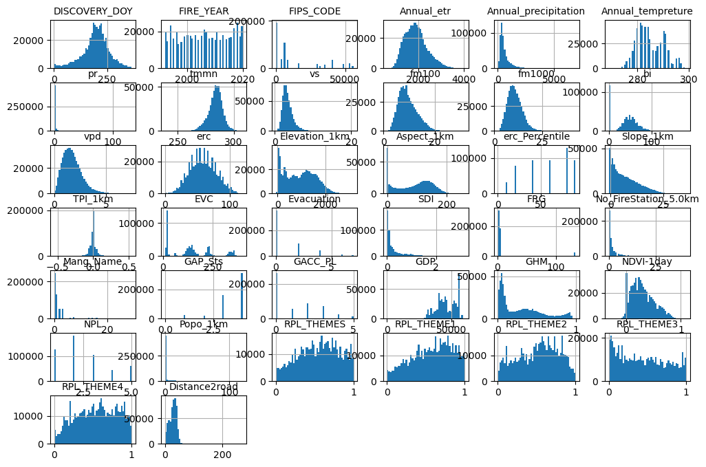
The data set includes meteorological, topological, social, and fire management variables:

• ‘DISCOVERY_DOY’: Day of year on which the fire was discovered or confirmed to exist

• ‘FIRE_YEAR’: Calendar year in which the fire was discovered or confirmed to exist

• ‘STATE’: Two-letter alphabetic code for the state in which the fire burned (or originated), based on fire report

• ‘FIPS_CODE’: Five digit code from the Federal Information Process Standards publication 6-4 for representation of counties and equivalent entities, based on the nominal designation in the fire report.

• ‘Annual_etr’: Annual total reference evaporatranspiration (mm)

• ‘Annual_temperature’: Annual average temperature (K)

• ‘pr’ : Precipitation amount (mm)

• ‘tmmn’: Minimum temperature (K)

• ‘vs’: Wind velocity at 10 m above ground (m/s)

• ‘fm100’: 100-hour dead fuel moisture (%)

• ‘fm1000’: 1000-hour dead fuel moisture (%)

• ‘bi’: Burning index (NFDRS fire danger index)

• ‘vpd’: Mean vapor pressure deficit (kPa)

• ‘erc’: Energy release component (NFDRS fire danger index)

• ‘Elevation_1km’: Average elevation in 1 km radius around the ignition point

• ‘Aspect_1km’: Average aspect in 1 km radius around the ignition point

• ‘erc_Percentile’: Percentile range of energy release component

• ‘Slope_1km’: Average slope in 1 km radius around the ignition point

• ‘TPI_1km’: Average Topographic Position Index in 1 km radius around the ignition point

• ‘EVC’: Existing Vegetation Cover - vertically projected percent cover of the live canopy layer for a specific area (%)

• ‘Evacuation’: Estimate ground transport time in hours from the fire ignition point to a definitive care facility (hospital)

• ‘SDI’: Suppression difficulty index (Rodriguez y Silva et al. 2020): relative difficulty of fire control

• ‘FRG’: Fire regime group - presumed historical fire regime

• ‘No_FireStation_5.0km’: Number of fire stations in a 5 km radius around the fire ignition point

• ‘Mang_Name’: The land manager or administrative agency standardized for the US

• ‘GAP_Sts’: GAP status code classifies management intent to conserve biodiversity

• ‘GACC_PL’: Geographic Area Coordination Center (GACC) Preparedness Level

• ‘GDP’: Annual Gross Domestic Product Per Capita

• ‘GHM’: Cumulative Measure of the human modification of lands within 1 km of the fire ignition point

• ‘NDVI-1day’: Normalized Difference Vegetation Index (NDVI) on the day prior to ignition

• ‘NPL’: National Preparedness Level

• ‘Popo_1km’: Average population density within a 1 km radius around the fire ignition point

• ‘RPL_THEMES’: Social Vulnerability Index (Overall Percentile Ranking)

• ‘RPL_THEME1’: Percentile Ranking for socioeconomic theme summary

• ‘RPL_THEME2’: Percentile Ranking for Household Composition theme summary

• ‘RPL_THEME3’: Percentile Ranking for Minority Status/Language theme

• ‘RPL_THEME4’: Precentile ranking for Housing Type/Transportion theme

• ‘Distance2road’: Distance to the nearest road

len(data)

519689

data.info()

<class 'pandas.core.frame.DataFrame'>
RangeIndex: 519689 entries, 0 to 519688
Data columns (total 40 columns):
 #   Column                Non-Null Count   Dtype  
---  ------                --------------   -----  
 0   DISCOVERY_DOY         519689 non-null  int64  
 1   FIRE_YEAR             519689 non-null  int64  
 2   STATE                 519689 non-null  object 
 3   FIPS_CODE             519689 non-null  float64
 4   NWCG_GENERAL_CAUSE    519689 non-null  object 
 5   Annual_etr            519689 non-null  int64  
 6   Annual_precipitation  519689 non-null  int64  
 7   Annual_tempreture     519689 non-null  float64
 8   pr                    519689 non-null  float64
 9   tmmn                  519689 non-null  float64
 10  vs                    519689 non-null  float64
 11  fm100                 519689 non-null  float64
 12  fm1000                519689 non-null  float64
 13  bi                    519689 non-null  float64
 14  vpd                   519689 non-null  float64
 15  erc                   519689 non-null  float64
 16  Elevation_1km         519689 non-null  float64
 17  Aspect_1km            519689 non-null  float64
 18  erc_Percentile        519689 non-null  float64
 19  Slope_1km             519689 non-null  float64
 20  TPI_1km               519689 non-null  float64
 21  EVC                   519689 non-null  float64
 22  Evacuation            519689 non-null  float64
 23  SDI                   519689 non-null  float64
 24  FRG                   519689 non-null  int64  
 25  No_FireStation_5.0km  519689 non-null  float64
 26  Mang_Name             519689 non-null  int64  
 27  GAP_Sts               519689 non-null  float64
 28  GACC_PL               519689 non-null  float64
 29  GDP                   519689 non-null  float64
 30  GHM                   519689 non-null  float64
 31  NDVI-1day             519689 non-null  float64
 32  NPL                   519689 non-null  float64
 33  Popo_1km              519689 non-null  float64
 34  RPL_THEMES            519689 non-null  float64
 35  RPL_THEME1            519689 non-null  float64
 36  RPL_THEME2            519689 non-null  float64
 37  RPL_THEME3            519689 non-null  float64
 38  RPL_THEME4            519689 non-null  float64
 39  Distance2road         519689 non-null  float64
dtypes: float64(32), int64(6), object(2)
memory usage: 158.6+ MB

firecauses = data['NWCG_GENERAL_CAUSE'].value_counts()
print(firecauses)

NWCG_GENERAL_CAUSE
Natural                                       168349
Missing data/not specified/undetermined       150427
Equipment and vehicle use                      48994
Debris and open burning                        40516
Recreation and ceremony                        38665
Arson/incendiarism                             28090
Smoking                                        13547
Misuse of fire by a minor                      11523
Power generation/transmission/distribution      6469
Fireworks                                       6373
Railroad operations and maintenance             3074
Other causes                                    2068
Firearms and explosives use                     1594
Name: count, dtype: int64

## Deal with some bad data 
data.loc[data["GHM"]<0.0,"GHM"] = np.nan
data.loc[data["SDI"]<0.0,"SDI"] = np.nan
data['FRG'] = data['FRG'].replace(-9999,np.nan)
data["RPL_THEMES"] = data["RPL_THEMES"].replace(-999.0,np.nan)
data["RPL_THEME1"] = data["RPL_THEME1"].replace(-999.0,np.nan)
data["RPL_THEME2"] = data["RPL_THEME2"].replace(-999.0,np.nan)
data["RPL_THEME3"] = data["RPL_THEME3"].replace(-999.0,np.nan)
data["RPL_THEME4"] = data["RPL_THEME4"].replace(-999.0,np.nan)

import matplotlib.pyplot as plt

# extra code – the next 5 lines define the default font sizes
plt.rc('font', size=10)
plt.rc('axes', labelsize=10, titlesize=10)
plt.rc('legend', fontsize=10)
plt.rc('xtick', labelsize=10)
plt.rc('ytick', labelsize=10)

data.hist(bins=50, figsize=(12, 8))
#save_fig("attribute_histogram_plots")  # extra code
plt.show()

data_cleaned = data.dropna().reset_index(drop=True)

Separate out the fires with no known cause

First, let’s separate all of the fires where NWCG_GENERAL_CAUSE has the label Missing data/not specified/undetermined.

data_sorted = data_cleaned.iloc[np.where(data_cleaned['NWCG_GENERAL_CAUSE'] == 'Missing data/not specified/undetermined')[0].tolist() +
                    np.where(data_cleaned['NWCG_GENERAL_CAUSE'] != 'Missing data/not specified/undetermined')[0].tolist()].reset_index(drop=True).copy()

data_sorted

	DISCOVERY_DOY	FIRE_YEAR	STATE	FIPS_CODE	NWCG_GENERAL_CAUSE	Annual_etr	Annual_precipitation	Annual_tempreture	pr	tmmn	...	GHM	NDVI-1day	NPL	Popo_1km	RPL_THEMES	RPL_THEME1	RPL_THEME2	RPL_THEME3	RPL_THEME4	Distance2road
0	1	2007	CA	6065.0	Missing data/not specified/undetermined	2359	100	292.0	0.0	277.799988	...	0.84	0.22	1.0	5.2191	0.261	0.167	0.424	0.427	0.256	38.5
1	1	2007	CA	6065.0	Missing data/not specified/undetermined	2452	110	291.0	0.0	275.899994	...	0.61	0.17	1.0	1.3687	0.927	0.969	0.940	0.846	0.607	38.3
2	1	2007	AZ	0.0	Missing data/not specified/undetermined	3146	135	292.0	0.0	273.100006	...	0.04	0.11	1.0	0.0000	0.504	0.829	0.535	0.046	0.394	36.2
3	1	2007	CA	6065.0	Missing data/not specified/undetermined	3546	20	297.0	0.0	277.100006	...	0.92	0.04	1.0	8.1135	0.611	0.498	0.653	0.594	0.688	37.5
4	1	2007	CA	6065.0	Missing data/not specified/undetermined	2486	92	292.0	0.0	277.799988	...	0.88	0.18	1.0	13.7651	0.939	0.833	0.879	0.822	0.875	38.8
...	...	...	...	...	...	...	...	...	...	...	...	...	...	...	...	...	...	...	...	...	...
518654	364	2003	CO	0.0	Arson/incendiarism	2222	390	284.0	0.0	263.500000	...	0.08	0.29	1.0	0.0007	0.464	0.560	0.089	0.688	0.695	16.8
518655	364	2003	CO	8043.0	Arson/incendiarism	1891	636	280.0	0.0	261.700012	...	0.06	0.37	1.0	0.0003	0.464	0.560	0.089	0.688	0.695	16.8
518656	365	2003	CA	6025.0	Recreation and ceremony	2846	63	298.0	0.0	286.500000	...	0.19	-0.00	1.0	0.0000	0.715	0.914	0.545	0.500	0.421	8.7
518657	365	2003	CA	0.0	Debris and open burning	1805	994	287.0	0.0	274.100006	...	0.39	0.02	1.0	0.4738	0.216	0.509	0.207	0.008	0.151	33.6
518658	365	2003	CA	6065.0	Equipment and vehicle use	2048	318	292.0	0.0	280.399994	...	0.81	0.11	1.0	1.1717	0.636	0.785	0.567	0.453	0.377	6.1

518659 rows × 40 columns

data_unknown = data_sorted.loc[data_sorted["NWCG_GENERAL_CAUSE"] == "Missing data/not specified/undetermined"].reset_index(drop=True).copy()
data_known = data_sorted.loc[data_sorted["NWCG_GENERAL_CAUSE"] != "Missing data/not specified/undetermined"].reset_index(drop=True).copy()

data_known["NWCG_GENERAL_CAUSE"].value_counts()

NWCG_GENERAL_CAUSE
Natural                                       168126
Equipment and vehicle use                      48895
Debris and open burning                        40450
Recreation and ceremony                        38498
Arson/incendiarism                             28035
Smoking                                        13510
Misuse of fire by a minor                      11508
Power generation/transmission/distribution      6453
Fireworks                                       6348
Railroad operations and maintenance             3062
Other causes                                    2064
Firearms and explosives use                     1584
Name: count, dtype: int64

Since only the first class is due to natural causes (typically ignition is due to lightning), and all the other categories are related to human activity, we can also label fires as being “natural” or “anthropogenic”. We’ll create a binary variable called “IsNatural” which has a value of 1 (True) if it is fire caused by natural causes or 0 (False) if it is a fire caused by any of the other causes related to human activity.

data_known["IsNatural"] = (data_known["NWCG_GENERAL_CAUSE"] == "Natural").astype(int)

data_known["IsNatural"].value_counts()

IsNatural
0    200407
1    168126
Name: count, dtype: int64

Data Pre-Processing

For decision trees and random forests, we generally don’t have to worry as much about scaling (compared with models like neural networks), since they work based on finding threshold values in the data sets.

from sklearn.preprocessing import OneHotEncoder, OrdinalEncoder
from sklearn.preprocessing import StandardScaler
from sklearn.pipeline import make_pipeline
from sklearn.compose import ColumnTransformer

causes = data_known[['NWCG_GENERAL_CAUSE']]
isnatural = data_known[["IsNatural"]]
features = data_known.copy().drop(["NWCG_GENERAL_CAUSE","IsNatural"],axis=1)
features_unknown = data_unknown.copy().drop(["NWCG_GENERAL_CAUSE"],axis=1)

We’ll create two labels for our data set. The first is a binary label, for whether the fire was caused by natural or anthropogenic causes.

y_binary = isnatural.to_numpy()

classnames_binary = ["Anthropogenic","Natural"]

The second set of labels will be multi-class, and include all of the possible causes for the fires included in the NWCG_GENERAL_CAUSE column.

ordenc = OrdinalEncoder()
y_multiclass = ordenc.fit_transform(causes)

classnames_multi = ordenc.categories_[0]
print(classnames_multi)

['Arson/incendiarism' 'Debris and open burning'
 'Equipment and vehicle use' 'Firearms and explosives use' 'Fireworks'
 'Misuse of fire by a minor' 'Natural' 'Other causes'
 'Power generation/transmission/distribution'
 'Railroad operations and maintenance' 'Recreation and ceremony' 'Smoking']

Now we will create the pipeline to transform the variables in the features dataframe as input to the model.

categorical_cols = ["STATE"]
numerical_cols = ['DISCOVERY_DOY', 'FIRE_YEAR', 'FIPS_CODE', 'Annual_etr', 'Annual_precipitation','Annual_tempreture', 
                  'pr', 'tmmn', 'vs', 'fm100', 'fm1000', 'bi', 'vpd', 'erc', 'Elevation_1km', 'Aspect_1km', 'erc_Percentile', 
                  'Slope_1km','TPI_1km', 'EVC', 'Evacuation', 'SDI', 'FRG', 'No_FireStation_5.0km','Mang_Name', 'GAP_Sts', 
                  'GACC_PL', 'GDP', 'GHM', 'NDVI-1day', 'NPL','Popo_1km', 'RPL_THEMES', 'RPL_THEME1', 'RPL_THEME2', 'RPL_THEME3',
                  'RPL_THEME4', 'Distance2road']

cat_pipeline = make_pipeline(OrdinalEncoder(),StandardScaler())
num_pipeline = make_pipeline(StandardScaler())

preprocessor = ColumnTransformer([
    ("n",num_pipeline,numerical_cols),
    ("c",cat_pipeline,categorical_cols)])

X_known = preprocessor.fit_transform(features)

We’ll use the same pipeline to transform the features associated with the unknown fires. In this case we will use transform rather than fit_transform. The difference is that the scalings and transformations will be based on the data in features (rather than features_unknown) so we will end up performing exactly the same scalings and transformations on both data sets. This is important because the models that we will train later will depend on these scalings and transformations being consistent across both data sets.

X_unknown = preprocessor.transform(features_unknown)

print(X_known.shape,X_unknown.shape)

(368533, 39) (150126, 39)

featurenames = preprocessor.get_feature_names_out()
print(featurenames)

['n__DISCOVERY_DOY' 'n__FIRE_YEAR' 'n__FIPS_CODE' 'n__Annual_etr'
 'n__Annual_precipitation' 'n__Annual_tempreture' 'n__pr' 'n__tmmn'
 'n__vs' 'n__fm100' 'n__fm1000' 'n__bi' 'n__vpd' 'n__erc'
 'n__Elevation_1km' 'n__Aspect_1km' 'n__erc_Percentile' 'n__Slope_1km'
 'n__TPI_1km' 'n__EVC' 'n__Evacuation' 'n__SDI' 'n__FRG'
 'n__No_FireStation_5.0km' 'n__Mang_Name' 'n__GAP_Sts' 'n__GACC_PL'
 'n__GDP' 'n__GHM' 'n__NDVI-1day' 'n__NPL' 'n__Popo_1km' 'n__RPL_THEMES'
 'n__RPL_THEME1' 'n__RPL_THEME2' 'n__RPL_THEME3' 'n__RPL_THEME4'
 'n__Distance2road' 'c__STATE']

Training, validation, and test split

Then we will split the data where the cause of the fire is known into training, validation, and test data sets.

from sklearn.model_selection import train_test_split

We’ll create an index z as input to the train_test_split function. This way, we can select either the binary or multiclass labels for our training, validation, and test data sets.

z_known = np.arange(0,X_known.shape[0])

X_train, X_val_test, z_train, z_val_test = train_test_split(X_known,z_known,test_size = 0.2, random_state = 42)
X_val, X_test, z_val, z_test = train_test_split(X_val_test, z_val_test ,test_size = 0.5, random_state = 42)

z_train.shape

(294826,)

y_multiclass_train = y_multiclass[z_train].ravel()
y_multiclass_test = y_multiclass[z_test].ravel()
y_multiclass_val = y_multiclass[z_val].ravel()

y_binary_train = y_binary[z_train].ravel()
y_binary_test = y_binary[z_test].ravel()
y_binary_val = y_binary[z_val].ravel()

print(X_train.shape,X_val.shape,X_test.shape)
print(y_binary_train.shape,y_binary_val.shape,y_binary_test.shape)

(294826, 39) (36853, 39) (36854, 39)
(294826,) (36853,) (36854,)

Train logistic regression (natural vs. human causes)

from sklearn.linear_model import LogisticRegression
log_reg = LogisticRegression(solver="lbfgs", random_state=42)

log_reg.fit(X_train, y_binary_train)

LogisticRegression(random_state=42)

In a Jupyter environment, please rerun this cell to show the HTML representation or trust the notebook.
On GitHub, the HTML representation is unable to render, please try loading this page with nbviewer.org.

log_reg.score(X_train,y_binary_train)

0.8811231031184495

log_reg.score(X_val,y_binary_val)

0.882479038341519

y_train_predicted = log_reg.predict(X_train)
y_val_predicted = log_reg.predict(X_val)

from sklearn.metrics import confusion_matrix
from sklearn.metrics import ConfusionMatrixDisplay

confusion_matrix(y_binary_val, y_val_predicted)

array([[17695,  2302],
       [ 2029, 14827]])

confusion_matrix(y_binary_train, y_train_predicted)

array([[142077,  18472],
       [ 16576, 117701]])

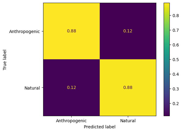
ConfusionMatrixDisplay.from_predictions(y_binary_train, y_train_predicted,normalize='true',display_labels=classnames_binary)

<sklearn.metrics._plot.confusion_matrix.ConfusionMatrixDisplay at 0x16bab27c0>

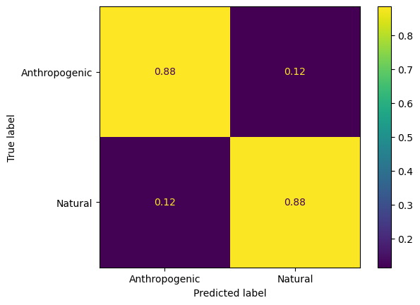
ConfusionMatrixDisplay.from_predictions(y_binary_val, y_val_predicted,normalize='true',display_labels=classnames_binary)

<sklearn.metrics._plot.confusion_matrix.ConfusionMatrixDisplay at 0x31faa2c40>

from sklearn.metrics import accuracy_score, precision_score, recall_score, f1_score

Accuracy is defined as

\(\frac{TP+TN}{TP+TN+FP+FN}\)

where

• TP = True positive

• TN = True negative

• FP = False positive

• FN = False negative

When accuracy = 1.0, this indicates a perfect classifier, while 0.0 indicates no skill. However, accuracy can be missleading if our classes are imbalanced.

accuracy_score(y_binary_val,y_val_predicted)

0.882479038341519

Precision tells us how accurately the classifier is able to identify objects of a specific class. It is defined as

\( precision = \frac{TP}{TP + FP}\).

High precision means that we will tolerate false negatives, but have as few false positives as possible.

precision_score(y_binary_val, y_val_predicted)

0.8656080331601378

Recall tells us how many of the objects of a class are correctly identified. It is defined as

\(recall = \frac{TP}{TP+FN}\)

High recall means that we will tolerate false positives, but try to have as few false negatives as possible.

recall_score(y_binary_val, y_val_predicted)

0.8796274323682961

Finally, if we want to find a balance between precision and recall, we can evaluate the F1 score:

\(F_{1} = \frac{2}{recall^{-1}+precision^{-1}}\)

f1_score(y_binary_val, y_val_predicted)

0.8725614241577166

ROC curve

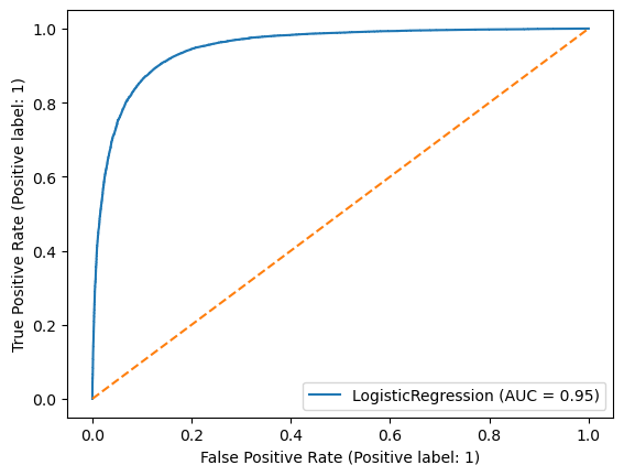
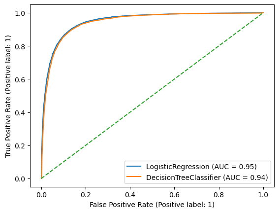
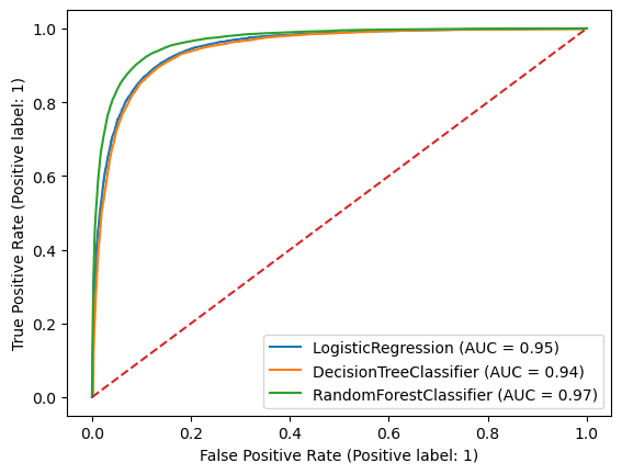
The Reciever Operator Characteristic (ROC) curve can be used to evaluate the performance of a binary classifier. Because there is a trade-off between true positives and false positives depending on where we set the threshold for identifying the two classes, the ROC curve can visualize this trade-off. A classifier with no skill would line on the diagnol dashed line, and a perfect classifier would have a curve reaching the top-left corner of the plot.

from sklearn.metrics import RocCurveDisplay

svc_disp = RocCurveDisplay.from_estimator(log_reg, X_val, y_binary_val)
plt.plot(np.arange(0,1.1,0.1),np.arange(0,1.1,0.1),linestyle='--')
plt.show()

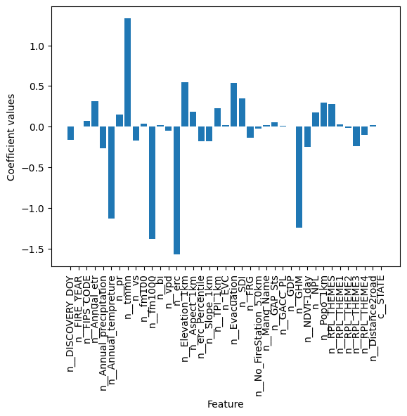
Importance of different features for logistic regression

coefficients = log_reg.coef_
coefficients.shape

(1, 39)

x = plt.bar(featurenames,coefficients[0,:])
plt.ylabel("Coefficient values")
plt.xlabel("Feature")
plt.xticks(rotation=90)
plt.show()

Train a decision tree classifier

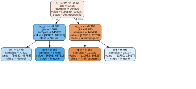
from sklearn.tree import DecisionTreeClassifier

tree_clf = DecisionTreeClassifier(max_depth=2, random_state=42)
tree_clf.fit(X_train, y_binary_train)

DecisionTreeClassifier(max_depth=2, random_state=42)

In a Jupyter environment, please rerun this cell to show the HTML representation or trust the notebook.
On GitHub, the HTML representation is unable to render, please try loading this page with nbviewer.org.

!pip install graphviz

Requirement already satisfied: graphviz in /opt/anaconda3/envs/ML4Climate2025/lib/python3.8/site-packages (0.20.3)

We can directly visualize the decision tree using the graphviz library, and look at what thresholds it is using at each node.

from graphviz import Source
from sklearn.tree import export_graphviz

export_graphviz(
        tree_clf,
        out_file="decision_tree.dot",
        feature_names=featurenames,
        class_names=classnames_binary,
        rounded=True,
        filled=True
    )

# Read the dot file 
with open("decision_tree.dot") as f:
    dot_graph = f.read()

# Adjust dpi for scaling
dot_graph = 'digraph Tree {\ndpi=50;\n' + dot_graph.split('\n', 1)[1]

Source(dot_graph)

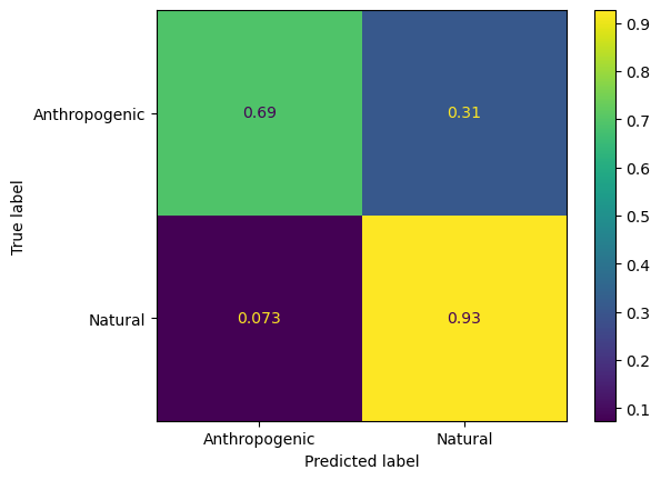
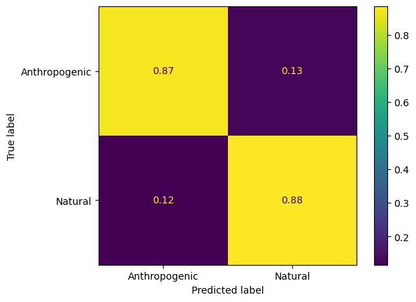
Let’s train decision trees with greater max_depth and see how they perform on the validation data set.

depths = [2,10,20,50]
trained_decisiontrees = []

for i in depths:
    tree_clf = DecisionTreeClassifier(max_depth=i, random_state=42)
    trained_decisiontrees.append(tree_clf.fit(X_train, y_binary_train))

y_val_predicted = trained_decisiontrees[0].predict(X_val)

y_val_predicted

array([1, 0, 1, ..., 1, 1, 0])

ConfusionMatrixDisplay.from_estimator(trained_decisiontrees[0],X_val,y_binary_val,normalize='true',display_labels=classnames_binary)

<sklearn.metrics._plot.confusion_matrix.ConfusionMatrixDisplay at 0x31fb7cf10>

ConfusionMatrixDisplay.from_estimator(trained_decisiontrees[1],X_val,y_binary_val,normalize='true',display_labels=classnames_binary)

<sklearn.metrics._plot.confusion_matrix.ConfusionMatrixDisplay at 0x15f41ccd0>

ConfusionMatrixDisplay.from_estimator(trained_decisiontrees[2],X_val,y_binary_val,normalize='true',display_labels=classnames_binary)

<sklearn.metrics._plot.confusion_matrix.ConfusionMatrixDisplay at 0x16ba590d0>

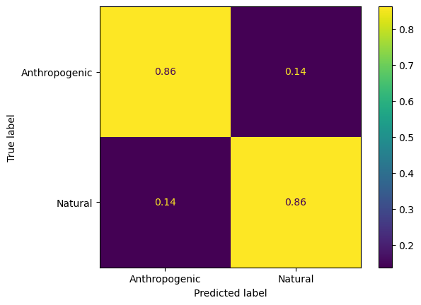
ConfusionMatrixDisplay.from_estimator(trained_decisiontrees[3],X_val,y_binary_val,normalize='true',display_labels=classnames_binary)

<sklearn.metrics._plot.confusion_matrix.ConfusionMatrixDisplay at 0x16baac460>

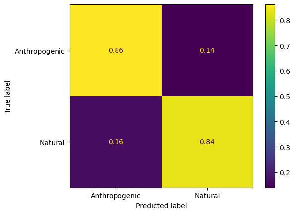
We can compare the performance of a the trained decision tree to logistic regression.

ax = plt.gca()
svc_disp = RocCurveDisplay.from_estimator(log_reg, X_val, y_binary_val,ax=ax)
svc_disp = RocCurveDisplay.from_estimator(trained_decisiontrees[1], X_val, y_binary_val,ax=ax)
ax.plot(np.arange(0,1.1,0.1),np.arange(0,1.1,0.1),linestyle='--')
plt.show()

Train a random forest classifier

A random forest is an ensemble of decision trees. Each decision tree is grown on a different sub-sample of the data set, and their ensemble vote is typically better than that of a single decision tree. They are quite powerful methods that are still used widely in environmental science and climate research, and are particularly good on tabular data sets. They can however be rather slow to train if the training data set is large.

from sklearn.ensemble import RandomForestClassifier

rnd_clf = RandomForestClassifier(n_estimators=100, random_state=42)

rnd_clf.fit(X_train,y_binary_train)

RandomForestClassifier(random_state=42)

In a Jupyter environment, please rerun this cell to show the HTML representation or trust the notebook.
On GitHub, the HTML representation is unable to render, please try loading this page with nbviewer.org.

ConfusionMatrixDisplay.from_estimator(rnd_clf,X_val,y_binary_val,normalize='true',display_labels=classnames_binary)

<sklearn.metrics._plot.confusion_matrix.ConfusionMatrixDisplay at 0x31fb309a0>

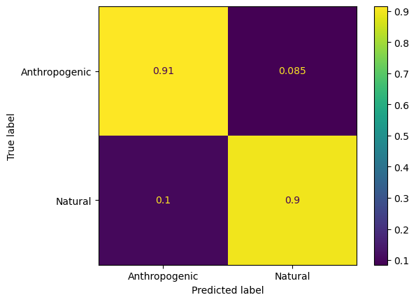
We can compare the trained random forest with the decision tree and logistic regression. In this case the random forest does give us some improvement.

ax = plt.gca()
svc_disp = RocCurveDisplay.from_estimator(log_reg, X_val, y_binary_val,ax=ax)
svc_disp = RocCurveDisplay.from_estimator(trained_decisiontrees[1], X_val, y_binary_val,ax=ax)
svc_disp = RocCurveDisplay.from_estimator(rnd_clf, X_val, y_binary_val,ax=ax)
ax.plot(np.arange(0,1.1,0.1),np.arange(0,1.1,0.1),linestyle='--')
plt.show()

Feature importance

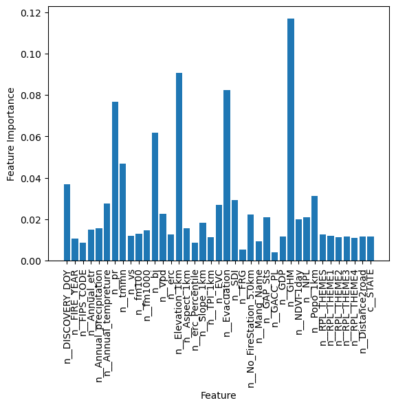
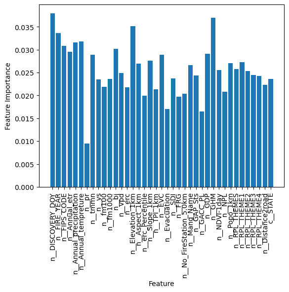
With random forests, we can also get some ideas of which features are the most important for our classifier.

rnd_clf.feature_importances_

array([0.03678424, 0.010523  , 0.00857334, 0.01493381, 0.01567114,
       0.02743097, 0.07660563, 0.04684962, 0.01184543, 0.01285308,
       0.01466824, 0.0617133 , 0.02268836, 0.01251963, 0.09073005,
       0.01565229, 0.00856963, 0.01815727, 0.01130637, 0.02685617,
       0.0824383 , 0.02938211, 0.00523526, 0.02220977, 0.0093963 ,
       0.02086468, 0.00383213, 0.01152713, 0.11698223, 0.01991252,
       0.02078227, 0.03123305, 0.01249902, 0.01197704, 0.01121416,
       0.01153355, 0.01094183, 0.0116142 , 0.01149288])

x = plt.bar(featurenames,rnd_clf.feature_importances_)
plt.ylabel("Feature Importance")
plt.xlabel("Feature")
plt.xticks(rotation=90)
plt.show()

Multiclass classification with the Random Forest

rnd_multiclass_clf = RandomForestClassifier(n_estimators=30, random_state=42, class_weight = "balanced")

import time

start = time.time()
rnd_multiclass_clf.fit(X_train,y_multiclass_train)
end = time.time()
print(end - start)

31.467910051345825

# Print the depth of each tree
for i, tree in enumerate(rnd_multiclass_clf.estimators_):
    print(f"Tree {i+1}: Depth = {tree.get_depth()}")  

Tree 1: Depth = 45
Tree 2: Depth = 46
Tree 3: Depth = 49
Tree 4: Depth = 43
Tree 5: Depth = 50
Tree 6: Depth = 50
Tree 7: Depth = 48
Tree 8: Depth = 48
Tree 9: Depth = 44
Tree 10: Depth = 59
Tree 11: Depth = 50
Tree 12: Depth = 46
Tree 13: Depth = 51
Tree 14: Depth = 51
Tree 15: Depth = 43
Tree 16: Depth = 48
Tree 17: Depth = 47
Tree 18: Depth = 47
Tree 19: Depth = 46
Tree 20: Depth = 51
Tree 21: Depth = 50
Tree 22: Depth = 43
Tree 23: Depth = 44
Tree 24: Depth = 47
Tree 25: Depth = 48
Tree 26: Depth = 50
Tree 27: Depth = 48
Tree 28: Depth = 47
Tree 29: Depth = 48
Tree 30: Depth = 47

This can be slow. If we want to train a model and save the trained weights, we can use pickle so we don’t need to train this again.

import pickle

filename = 'rnd_multiclass_clf.pkl'
with open(filename, 'wb') as file:
    pickle.dump(rnd_multiclass_clf, file)

Then we can load the weights in later using the following lines.

loaded_model = pickle.load(open(filename, 'rb'))

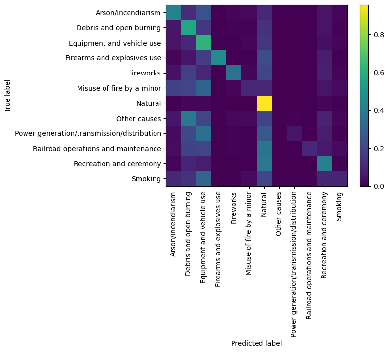
We can evaluate the trained multi-class classifier.

cmp = ConfusionMatrixDisplay.from_estimator(rnd_multiclass_clf,X_val,y_multiclass_val,normalize='true',
                                      display_labels=classnames_multi, xticks_rotation="vertical",include_values=False);

from sklearn.metrics import classification_report

y_val_predicted = rnd_multiclass_clf.predict(X_val)

print(classification_report(y_val_predicted,y_multiclass_val,target_names = classnames_multi))

                                            precision    recall  f1-score   support

                        Arson/incendiarism       0.43      0.53      0.47      2214
                   Debris and open burning       0.57      0.51      0.54      4606
                 Equipment and vehicle use       0.62      0.51      0.56      6016
               Firearms and explosives use       0.46      0.96      0.62        72
                                 Fireworks       0.36      0.59      0.45       389
                 Misuse of fire by a minor       0.10      0.34      0.16       354
                                   Natural       0.96      0.80      0.87     20021
                              Other causes       0.00      0.08      0.01        13
Power generation/transmission/distribution       0.05      0.49      0.10        67
       Railroad operations and maintenance       0.11      0.69      0.18        49
                   Recreation and ceremony       0.42      0.59      0.49      2681
                                   Smoking       0.10      0.36      0.16       371

                                  accuracy                           0.68     36853
                                 macro avg       0.35      0.54      0.38     36853
                              weighted avg       0.76      0.68      0.71     36853

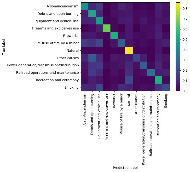
The classes are pretty imbalanced, so one approach we can try is over-sampling the classes that are not well-represented.

!pip install imbalanced-learn

Requirement already satisfied: imbalanced-learn in /opt/anaconda3/envs/ML4Climate2025/lib/python3.8/site-packages (0.12.4)
Requirement already satisfied: numpy>=1.17.3 in /opt/anaconda3/envs/ML4Climate2025/lib/python3.8/site-packages (from imbalanced-learn) (1.24.3)
Requirement already satisfied: scipy>=1.5.0 in /opt/anaconda3/envs/ML4Climate2025/lib/python3.8/site-packages (from imbalanced-learn) (1.10.1)
Requirement already satisfied: scikit-learn>=1.0.2 in /opt/anaconda3/envs/ML4Climate2025/lib/python3.8/site-packages (from imbalanced-learn) (1.3.2)
Requirement already satisfied: joblib>=1.1.1 in /opt/anaconda3/envs/ML4Climate2025/lib/python3.8/site-packages (from imbalanced-learn) (1.4.2)
Requirement already satisfied: threadpoolctl>=2.0.0 in /opt/anaconda3/envs/ML4Climate2025/lib/python3.8/site-packages (from imbalanced-learn) (3.5.0)

from imblearn.over_sampling import SMOTE

The SMOTE algorithm interpolates between the points in each class in order to create new examples similar to the training data set in order to augment the data set.

sm = SMOTE(random_state=42)

X_resampled, y_resampled = sm.fit_resample(X_train,y_multiclass_train)

This makes our data set much larger however.

X_resampled.shape

(1611324, 39)

X_resampled.shape[0]/X_train.shape[0]

5.465338877846595

We will randomly sample the resampled data set so that we will have the same size as the original training data set.

z = np.arange(0,X_resampled.shape[0])
idx = np.random.choice(z, size=X_train.shape[0], replace=False)
X_balanced = X_resampled[idx]
y_balanced = y_resampled[idx]

rnd_multiclass_clf2 = RandomForestClassifier(n_estimators=30, random_state=42, class_weight = "balanced")

start = time.time()
rnd_multiclass_clf2.fit(X_balanced,y_balanced)
end = time.time()
print(end - start)

50.9616539478302

cmp = ConfusionMatrixDisplay.from_estimator(rnd_multiclass_clf2,X_val,y_multiclass_val,normalize='true',
                                      display_labels=classnames_multi, xticks_rotation="vertical",include_values=False);

y_val_predicted_oversampled = rnd_multiclass_clf2.predict(X_val)

print(classification_report(y_val_predicted_oversampled,y_multiclass_val,target_names = classnames_multi))

                                            precision    recall  f1-score   support

                        Arson/incendiarism       0.42      0.46      0.44      2529
                   Debris and open burning       0.51      0.54      0.52      3835
                 Equipment and vehicle use       0.47      0.54      0.51      4268
               Firearms and explosives use       0.67      0.32      0.43       314
                                 Fireworks       0.53      0.33      0.41      1050
                 Misuse of fire by a minor       0.26      0.22      0.23      1349
                                   Natural       0.86      0.89      0.88     16249
                              Other causes       0.17      0.07      0.10       507
Power generation/transmission/distribution       0.27      0.16      0.20      1004
       Railroad operations and maintenance       0.32      0.17      0.22       606
                   Recreation and ceremony       0.53      0.50      0.51      4034
                                   Smoking       0.19      0.24      0.22      1108

                                  accuracy                           0.63     36853
                                 macro avg       0.43      0.37      0.39     36853
                              weighted avg       0.63      0.63      0.63     36853

x = plt.bar(featurenames,rnd_multiclass_clf2.feature_importances_)
plt.ylabel("Feature Importance")
plt.xlabel("Feature")
plt.xticks(rotation=90)
plt.show()

Exercises

Try these short extensions of the tutorial. Each one reuses a method, model, or library we covered above, applied to a different variable, split, or setting. Work in new cells below.

1. Class balance. Using value_counts() on data_known["NWCG_GENERAL_CAUSE"], make a bar plot (.plot.bar()) of how many fires there are of each cause. Which three causes are the most common, and which is the rarest?

2. A different tree depth. The tutorial trained decision trees at depths 2, 10, 20, and 50. Train one more DecisionTreeClassifier with max_depth=5 on the binary target and print its .score() on the validation set. Where does its accuracy fall relative to the depth-2 and depth-10 trees?

3. Metrics for the decision tree. Using precision_score, recall_score, and f1_score, compute these three metrics for the depth-10 decision tree (trained_decisiontrees[1]) on the validation set, and compare them to the logistic-regression values from the tutorial.

4. Number of trees. Retrain the binary RandomForestClassifier twice, once with n_estimators=30 and once with n_estimators=200 (keep random_state=42). Print the validation accuracy of each. Does adding more trees keep improving the score?

5. Top features. The tutorial plotted rnd_clf.feature_importances_ as a bar chart. Instead, build a pandas Series from rnd_clf.feature_importances_ indexed by featurenames, sort it in descending order, and print the 5 most important features for the binary classifier.

6. Confusion matrix on the test set. The tutorial evaluated on the validation set. Use ConfusionMatrixDisplay.from_estimator (or confusion_matrix) to show the binary random forest’s performance on the held-out test set (X_test, y_binary_test) instead. Are the results similar to the validation set?

7. ROC on the test set. Plot the ROC curve of the binary random forest (rnd_clf) on the test set using RocCurveDisplay.from_estimator, and add the diagonal no-skill line as in the tutorial.

8. Does class weighting matter? The multiclass forest used class_weight="balanced". Train a second multiclass RandomForestClassifier with the same settings but class_weight=None, and compare the two with classification_report. Which classes change the most?

9. Predict the unknown fires. Use the trained multiclass forest (rnd_multiclass_clf) to predict causes for the fires with unknown cause (X_unknown). Turn the predictions back into class names with classnames_multi and use value_counts() to show how many unknown fires are predicted for each cause.

10. Save and reload a model. Using pickle, save your binary random forest rnd_clf to a file, load it back into a new variable, and confirm that the reloaded model gives the same predictions on X_val as the original (e.g. with np.array_equal).