GANs and Diffusion Models

The previous page framed generative modeling as predicting distributions of outputs. This page introduces the first two of three state-of-the-art generative architectures, the generative adversarial network (GAN) and the diffusion model, and surveys how they are used in climate and environmental science. We will:

• See how generative models learn the underlying distribution of the data rather than a decision boundary.

• Understand the generator vs. discriminator game that trains a GAN.

• Understand forward noising and learned denoising in diffusion models.

• Survey applications: downscaling, anomaly detection, and ensemble weather forecasting.

Learning the distribution, not the boundary

Think back to classification. A discriminative model looks at examples of, say, dogs and cats and learns where to put the decision boundary between the classes: on this side, probably a dog; on that side, probably a cat. A generative model asks a harder question: what is the underlying distribution that dog examples are drawn from, and likewise for cats? If we learn that distribution, we can do more than classify. We can draw new samples from it: completely new images of dogs that were never in the training set but are consistent with what the model learned a dog to be.

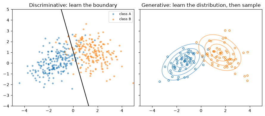
The toy example below makes the contrast concrete with two point clouds in two dimensions. The discriminative model (a logistic regression) only learns the line that separates them. The generative model fits a Gaussian distribution to each class, and can then generate brand new points from those fits.

import numpy as np
import matplotlib.pyplot as plt
from sklearn.linear_model import LogisticRegression

rng = np.random.default_rng(0)

n = 200
Xa = rng.multivariate_normal([-1.5, 0.0], [[1.0, 0.5], [0.5, 1.0]], n)
Xb = rng.multivariate_normal([1.5, 1.0], [[1.0, -0.3], [-0.3, 1.0]], n)
X = np.vstack([Xa, Xb])
y = np.r_[np.zeros(n), np.ones(n)]

clf = LogisticRegression().fit(X, y)

def gauss_pdf(pts, mu, cov):
    "evaluate a 2-D Gaussian density at an array of points"
    d = pts - mu
    inv = np.linalg.inv(cov)
    z = np.einsum("ni,ij,nj->n", d, inv, d)
    return np.exp(-0.5 * z) / (2 * np.pi * np.sqrt(np.linalg.det(cov)))

gx, gy = np.meshgrid(np.linspace(-5, 5, 200), np.linspace(-4, 5, 200))
grid = np.column_stack([gx.ravel(), gy.ravel()])

fig, axes = plt.subplots(1, 2, figsize=(9, 4), sharex=True, sharey=True)

# left: the discriminative view
p = clf.predict_proba(grid)[:, 1].reshape(gx.shape)
axes[0].contour(gx, gy, p, levels=[0.5], colors="k")
axes[0].scatter(*Xa.T, s=10, alpha=0.5, label="class A")
axes[0].scatter(*Xb.T, s=10, alpha=0.5, label="class B")
axes[0].set_title("Discriminative: learn the boundary")
axes[0].legend(fontsize=8)

# right: the generative view: fit a Gaussian per class, then sample from it
new_pts = []
for Xc, color in [(Xa, "tab:blue"), (Xb, "tab:orange")]:
    mu, cov = Xc.mean(axis=0), np.cov(Xc.T)
    dens = gauss_pdf(grid, mu, cov).reshape(gx.shape)
    axes[1].contour(gx, gy, dens, levels=4, colors=color, alpha=0.5)
    fresh = rng.multivariate_normal(mu, cov, 60)
    new_pts.append(fresh)
    axes[1].scatter(*fresh.T, s=18, facecolors="none", edgecolors=color)
axes[1].set_title("Generative: learn the distribution, then sample")
plt.tight_layout(); plt.show()

gen = np.vstack(new_pts)
gen_labels = np.r_[np.zeros(60), np.ones(60)]
agree = (clf.predict(gen) == gen_labels).mean()
print(f"fraction of newly generated points the classifier assigns "
      f"to the intended class: {agree:.2f}")

fraction of newly generated points the classifier assigns to the intended class: 0.97

On the left, everything the model knows is one curve. On the right, the model has an explicit density for each class, and the open circles are new samples that never existed in the training data. The printed check confirms the two views are consistent: nearly all generated points fall on the correct side of the discriminative boundary. Real data are far too complex for a single Gaussian per class, of course. The architectures below exist to learn much more flexible distributions, but the goal is exactly the one in the right panel.

1) Generative adversarial networks

A GAN trains two networks against each other:

• The generator receives a vector of random noise and turns it into a fake sample (an image, a rain field, …).

• The discriminator receives either a fake sample from the generator or a real one from the training set, and must decide which it is.

Both are trained simultaneously: the generator is optimized to fool the discriminator, and the discriminator to catch the generator. As the discriminator gets sharper, the generator is forced to make its fakes ever more realistic, and by the end it has effectively learned the underlying data distribution. Trained on photographs of faces, GANs produce the famous “deep fake” portraits of people who do not exist; trained on birds or clothing, they generate new, unseen but plausible birds and shirts.

GANs have become somewhat less popular in the last few years, displaced by the diffusion models below, partly because balancing two competing networks makes them notoriously tricky to train. But they remain fast at inference and widely used.

Application: downscaling

Downscaling, going from low resolution to high resolution, is the motivating problem from the previous page, and a natural GAN application. RainScaleGAN (Iotti et al. 2025) is a conditional GAN for rainfall downscaling: the generator receives the coarse resolution rainfall field as conditioning information along with the noise vector, and produces a plausible high resolution field; the discriminator sees either that generated field or the true high resolution field. Because the generator also takes noise, one coarse field can be downscaled many times to get an ensemble of plausible fine scale rainfall fields, exactly the uncertainty-aware output we argued for earlier.

Application: anomaly detection

A generative model knows what normal data look like, so it can flag what it cannot explain. Li et al. (2023) used GANs for real time monitoring of water distribution systems: trained on multi-parameter, multi-site water quality records, the model detects contamination events as anomalous signals that depart from the learned distribution, enabling automated monitoring without hand-labeled examples of every possible contamination.

2) Diffusion models

Diffusion probabilistic models have largely taken over from GANs as the state of the art. The idea has two halves:

• Forward process: take a training sample and gradually add noise to it, step by step, until nothing but noise remains.

• Reverse process: train a network to undo one step of noising. Starting from pure noise and applying the learned denoiser step by step then generates a brand new sample from the data distribution.

Compared to GANs, diffusion models are easier to train (one network, no adversarial balancing act) and generally produce better samples. Their principle is also rooted in ideas from statistical physics, which gives them a more physically grounded interpretation. The price is slow inference: a sample requires many denoising steps rather than one forward pass, and much current research aims at making both training and sampling faster.

The forward half needs no training at all; here it is on a toy two moons dataset.

from sklearn.datasets import make_moons

Xm, _ = make_moons(n_samples=2000, noise=0.05, random_state=0)
Xm = (Xm - Xm.mean(axis=0)) / Xm.std(axis=0)

T = 50
betas = np.linspace(1e-4, 0.25, T)          # noise added at each step
alphas = 1 - betas
abar = np.cumprod(alphas)                    # how much signal survives to step t

fig, axes = plt.subplots(1, 4, figsize=(11, 2.8), sharex=True, sharey=True)
for ax, t in zip(axes, [0, 5, 15, T - 1]):
    eps = rng.standard_normal(Xm.shape)
    xt = np.sqrt(abar[t]) * Xm + np.sqrt(1 - abar[t]) * eps
    ax.scatter(*xt.T, s=4, alpha=0.4)
    ax.set_title(f"step t = {t}")
fig.suptitle("Forward diffusion: data dissolve into Gaussian noise", y=1.02)
plt.tight_layout(); plt.show()

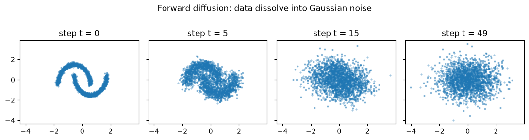
By the last step the two moons are gone: the points are indistinguishable from a standard Gaussian. Generation runs this movie backwards. For that we need the trained denoiser: a network that, given a noisy sample and the step number \(t\), predicts the noise that was added. We can build a miniature version with the tools we already have: an MLPRegressor taking \((x_1, x_2, t)\) as input and predicting the two components of the noise. Real diffusion models use deep architectures (typically U-Nets) and hundreds of steps, but the training loop is the same idea. While sampling we save snapshots along the way, so we can watch the reverse process mirror the forward one.

from sklearn.neural_network import MLPRegressor
from sklearn.neighbors import NearestNeighbors

# training set: (noisy point, t) -> the noise that was added
reps = 20
idx = rng.integers(0, len(Xm), len(Xm) * reps)
ts = rng.integers(0, T, len(idx))
eps = rng.standard_normal((len(idx), 2))
xt = (np.sqrt(abar[ts])[:, None] * Xm[idx]
      + np.sqrt(1 - abar[ts])[:, None] * eps)
feats = np.column_stack([xt, ts / T])

denoiser = MLPRegressor(hidden_layer_sizes=(64, 64), max_iter=200,
                        early_stopping=True, n_iter_no_change=5,
                        random_state=0).fit(feats, eps)

# reverse process: start from pure noise, denoise step by step
n_gen = 1000
x = rng.standard_normal((n_gen, 2))
snapshots = {T: x.copy()}                  # the starting pure noise
for t in reversed(range(T)):
    eps_hat = denoiser.predict(np.column_stack([x, np.full(n_gen, t / T)]))
    x = (x - betas[t] / np.sqrt(1 - abar[t]) * eps_hat) / np.sqrt(alphas[t])
    if t > 0:
        x = x + np.sqrt(betas[t]) * rng.standard_normal((n_gen, 2))
    if t in (15, 5, 0):
        snapshots[t] = x.copy()

fig, axes = plt.subplots(1, 4, figsize=(11, 2.8), sharex=True, sharey=True)
for ax, t in zip(axes, [T, 15, 5, 0]):
    ax.scatter(*snapshots[t].T, s=4, alpha=0.4, color="tab:orange")
    ax.set_title("start: pure noise" if t == T else f"step t = {t}")
fig.suptitle("Reverse diffusion: noise condenses back into data", y=1.02)
plt.tight_layout(); plt.show()

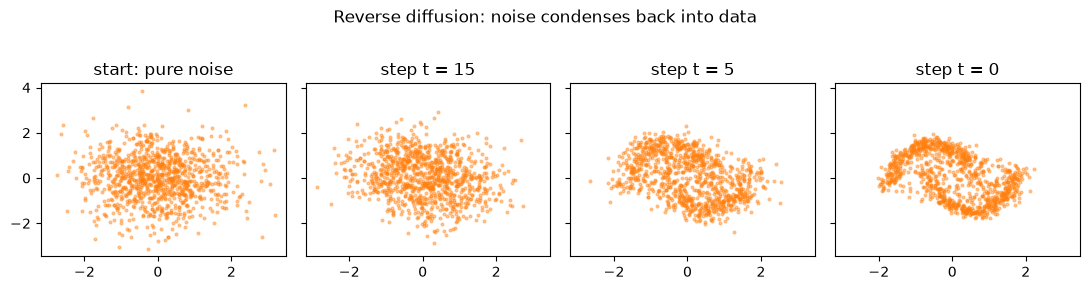
Read against the forward figure above, this is the same movie in reverse: the starting panel is indistinguishable from the forward process’s final one, at step \(t = 15\) the cloud is still nearly formless, by \(t = 5\) the two crescents have emerged from the blur, and the last five steps only sharpen them. Each panel is the same 1000 points partway through denoising. Comparing the finished samples against the real data:

fig, axes = plt.subplots(1, 2, figsize=(9, 3.6), sharex=True, sharey=True)
axes[0].scatter(*Xm.T, s=4, alpha=0.4)
axes[0].set_title("real data")
axes[1].scatter(*x.T, s=4, alpha=0.4, color="tab:orange")
axes[1].set_title("generated from pure noise")
plt.tight_layout(); plt.show()

d, _ = NearestNeighbors(n_neighbors=1).fit(Xm).kneighbors(x)
print(f"fraction of generated points within 0.25 of a real data point: "
      f"{(d < 0.25).mean():.2f}")

fraction of generated points within 0.25 of a real data point: 0.90

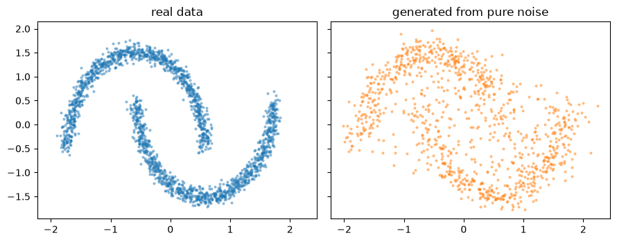
Starting from 1000 points of pure Gaussian noise, fifty passes through a small denoising network recover the two moons. The printed check quantifies it: about nine in ten generated points land within 0.25 of the data manifold, and none of them are copies of training points. This is the entire mechanism behind modern image generators, at toy scale.

Applications of diffusion models

Ensemble weather forecasting, without the ensemble. Weather forecasts are more accurate as ensembles: run the model many times from slightly different states and average, as we saw with the spread vs. skill plot on the previous page. But every extra member costs a full model run. Recent work at Google (SEEDS, Li et al. 2024) uses diffusion models for generative emulation of forecast ensembles: train on existing ensembles, then, given one or two forecasts, generate the rest of the ensemble by sampling instead of rerunning the physics. The generated ensembles reproduce the statistics of the true ensemble at a small fraction of the cost. Google DeepMind’s GenCast (see also the blog post) goes further: the weather model itself is a diffusion model, generating a full ensemble of possible future weather trajectories directly and predicting extreme conditions with state of the art accuracy.

Cyclone track prediction. A related Google DeepMind effort applies diffusion based ensembles to tropical cyclone tracks. Early in the forecast the generated tracks cluster tightly; further out they diverge, tracing the familiar cone of uncertainty. Across many storms the diffusion ensembles tracked the true cyclone paths better than the deterministic baseline, and the spread of tracks communicates the forecast’s confidence directly.

Summary

• Generative models learn the data distribution and can draw new samples from it; discriminative models only learn decision boundaries.

• GANs train a generator against a discriminator; powerful but tricky to balance. Conditional GANs downscale rainfall; the learned notion of “normal” supports anomaly detection.

• Diffusion models noise data forward and learn to denoise backward; easier to train, currently the state of the art, but slower at inference.

• In climate science these models downscale rainfall, flag anomalies, and produce cheap forecast ensembles and cyclone track cones.

The next page covers the third architecture, the variational autoencoder, and what its latent spaces offer scientific analysis.