
Supervised Regression#
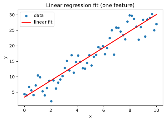
Regression predicts a continuous output from a set of input features. The setup mirrors classification: a model learns a function \(f\) mapping the feature matrix \(X\) to predictions \(\hat{Y} = f(X)\), and we minimize the difference between \(\hat{Y}\) and the ground-truth \(Y\). This page covers multiple linear regression, loss functions, over/under-fitting, benchmarking with \(R^2\), and regularization (Ridge and Lasso).
Multiple linear regression#
The simplest regressor writes the prediction as a weighted linear combination of the features plus a bias (intercept):
Each weight \(w_j\) is the (linear) importance of feature \(j\): how much \(\hat{y}\) changes per unit change in \(x_j\).
import numpy as np
import matplotlib.pyplot as plt
from sklearn.linear_model import LinearRegression

rng = np.random.default_rng(0)
x = np.linspace(0, 10, 60)
y = 2.5 * x + 4 + rng.normal(0, 3, x.size)     # true slope 2.5, intercept 4

lin = LinearRegression().fit(x.reshape(-1, 1), y)
print(f"learned slope = {lin.coef_[0]:.2f}, intercept = {lin.intercept_:.2f}")

plt.figure(figsize=(6, 4))
plt.scatter(x, y, s=20, label="data")
plt.plot(x, lin.predict(x.reshape(-1, 1)), "r", lw=2, label="linear fit")
plt.xlabel("x"); plt.ylabel("y"); plt.legend()
plt.title("Linear regression fit (one feature)")
plt.show()
learned slope = 2.66, intercept = 3.41
Loss functions for regression#
We measure error as the gap between truth \(y_i\) and prediction \(\hat{y}_i\):
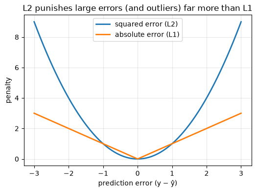
Mean Squared Error (MSE, L2 loss) — \(\frac{1}{N}\sum (y_i-\hat{y}_i)^2\). Squares the error, so large mistakes are penalized heavily. Units are squared.
Mean Absolute Error (MAE, L1 loss) — \(\frac{1}{N}\sum |y_i-\hat{y}_i|\). Keeps the original units and is less sensitive to outliers.
Root Mean Squared Error (RMSE) — \(\sqrt{\text{MSE}}\). Popular because it preserves the units of the target.
err = np.linspace(-3, 3, 200)
plt.figure(figsize=(6, 4))
plt.plot(err, err**2, lw=2, label="squared error (L2)")
plt.plot(err, np.abs(err), lw=2, label="absolute error (L1)")
plt.xlabel("prediction error (y − ŷ)"); plt.ylabel("penalty")
plt.title("L2 punishes large errors (and outliers) far more than L1")
plt.legend(); plt.grid(alpha=0.3)
plt.show()
Normal equation vs. gradient descent#
Linear regression has a closed-form solution, the normal equation:
It’s exact, but requires inverting an \(m \times m\) matrix — prohibitive when there are many features, and it needs \(X^\top X\) to be invertible. Gradient descent avoids the inversion, scales to large data sets that don’t fit in memory, and is what we use in practice for big problems.
Polynomial regression, underfitting and overfitting#
We can capture non-linear relationships by appending polynomial terms
(\(x^2, x^3, \dots\)) to the feature vector and still solving it as linear
regression (scikit-learn’s PolynomialFeatures does the appending).
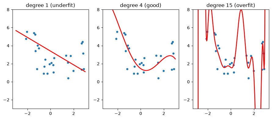
Model complexity has to be tuned:
Too simple (a straight line through curved data) → underfitting: poor on both training and test data.
Too complex (a very high-degree polynomial) → overfitting: it memorizes the training noise and generalizes badly.
Below we fit degree 1, 4, and 15 to the same noisy quadratic.
from sklearn.preprocessing import PolynomialFeatures
from sklearn.pipeline import make_pipeline

rng = np.random.default_rng(1)
xs = np.sort(rng.uniform(-3, 3, 30))
ys = 0.5 * xs**2 - xs + 2 + rng.normal(0, 1.5, xs.size)
grid = np.linspace(-3, 3, 200)

plt.figure(figsize=(9, 4))
for i, deg in enumerate([1, 4, 15]):
    model = make_pipeline(PolynomialFeatures(deg), LinearRegression()).fit(xs.reshape(-1, 1), ys)
    plt.subplot(1, 3, i + 1)
    plt.scatter(xs, ys, s=15)
    plt.plot(grid, model.predict(grid.reshape(-1, 1)), "r", lw=2)
    plt.ylim(-3, 8)
    plt.title(f"degree {deg}" + (" (underfit)" if deg == 1 else " (overfit)" if deg == 15 else " (good)"))
plt.tight_layout()
plt.show()
Benchmarking with \(R^2\)#
Step 1 — pick a metric (MSE, RMSE, MAE…).
Step 2 — report the coefficient of determination \(R^2\), the fraction of the variance in \(y\) that the model explains:
\(R^2 = 1\) is perfect; \(R^2 = 0\) is no better than predicting the mean; \(R^2 < 0\) means the model does worse than the mean. (Note \(R^2 \ne r\), the correlation coefficient.)
Step 3 — report on training, validation, and test sets separately. The test score estimates generalization — how the model will do on new, unseen data. A high training score with a low test score is the signature of overfitting.
from sklearn.model_selection import train_test_split
from sklearn.metrics import r2_score, mean_squared_error

# high-degree model to expose overfitting
X_ = xs.reshape(-1, 1)
Xtr, Xte, ytr, yte = train_test_split(X_, ys, test_size=0.4, random_state=0)
of = make_pipeline(PolynomialFeatures(15), LinearRegression()).fit(Xtr, ytr)

for name, Xs, ysub in [("train", Xtr, ytr), ("test", Xte, yte)]:
    pred = of.predict(Xs)
    print(f"{name:5s}  R^2 = {r2_score(ysub, pred):6.2f}   "
          f"RMSE = {np.sqrt(mean_squared_error(ysub, pred)):5.2f}")
train  R^2 =   0.98   RMSE =  0.38
test   R^2 = -2055712.29   RMSE = 2244.23
Regularization: Ridge and Lasso#
Regularization adds a penalty on the size of the weights to the loss, discouraging the model from fitting noise:
Ridge regression (L2) — penalizes \(\sum w_j^2\). Shrinks all coefficients toward zero but keeps every feature.
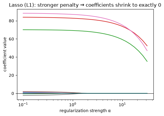
Lasso regression (L1) — penalizes \(\sum |w_j|\). Can drive some coefficients exactly to zero, performing implicit feature selection.
The plot below fits Lasso to a problem with many mostly-irrelevant features and increases the penalty strength \(\alpha\): watch the coefficients collapse to zero (sparse solution).
from sklearn.linear_model import Lasso
from sklearn.datasets import make_regression

Xr, yr = make_regression(n_samples=100, n_features=10, n_informative=3,
                         noise=10, random_state=0)
alphas = np.logspace(-1, 1.5, 30)
coefs = [Lasso(alpha=a, max_iter=10000).fit(Xr, yr).coef_ for a in alphas]

plt.figure(figsize=(6, 4))
plt.plot(alphas, coefs)
plt.xscale("log")
plt.xlabel("regularization strength α")
plt.ylabel("coefficient value")
plt.title("Lasso (L1): stronger penalty → coefficients shrink to exactly 0")
plt.axhline(0, color="k", lw=0.8)
plt.show()
Summary#
This page covered supervised regression — predicting a continuous target from a set of input features, using the same predict-then-minimize-a-loss recipe as classification.
Multiple linear regression predicts a weighted sum of the features plus a bias, \(\hat{y} = b + w_1 x_1 + \dots + w_m x_m = \mathbf{w}\cdot\mathbf{x} + b\). Each weight \(w_j\) is the linear importance of feature \(j\): how much the prediction changes per unit change in that feature.
Polynomial features (\(x^2, x^3, \dots\)) let the same linear machinery fit non-linear curves — you expand the feature vector and still solve a linear problem.
We fit the weights by minimizing a loss that measures how far predictions fall from the truth:
MSE / L2 squares the errors, so it punishes large mistakes hard and is sensitive to outliers; it has a clean closed-form solution.
MAE / L1 takes absolute errors, so it is more robust to outliers.
RMSE is the square root of MSE, reported to keep the error in the original units of the target.
Linear regression can be solved exactly with the normal equation \(\mathbf{w} = (X^\top X)^{-1} X^\top \mathbf{y}\), or iteratively with gradient descent when there are too many features to invert the matrix or the data don’t fit in memory.
Model complexity must be tuned between two failure modes: too simple underfits (poor on both training and test data), too complex overfits (memorizes training noise and generalizes badly). Always benchmark with \(R^2\) — the fraction of variance the model explains — on a held-out test set, never on the training data.
Regularization adds a penalty on the size of the weights to fight overfitting:
Ridge (L2) penalizes \(\sum w_j^2\), shrinking all coefficients toward zero but keeping every feature.
Lasso (L1) penalizes \(\sum |w_j|\) and can drive coefficients exactly to zero, performing implicit feature selection.
Next: Decision Trees and Random Forests, which drop the straight-line assumption entirely and partition the feature space into regions.