Tutorial on Global Temperature Trends with Deep Learning

Tutorial on Global Temperature Trends with Deep Learning#

Predicting global temperature from greenhouse gas concentrations#

This hands-on tutorial accompanies the Convolutional Neural Networks notes. Here we will look at an example of using a neural network to predict the global temperature given the global atmospheric concentrations of CO2 and CH4. This is based on this notebook developed by Weiwei Zhan.

import os
import numpy as np
import pandas as pd
import matplotlib.pyplot as plt
import xarray as xr
from glob import glob

import tensorflow as tf
from tensorflow import keras
from tensorflow.keras.models import Model, load_model
from tensorflow.keras.layers import *
from tensorflow.keras import Sequential

2025-07-31 03:17:35.012850: I tensorflow/core/util/port.cc:153] oneDNN custom operations are on. You may see slightly different numerical results due to floating-point round-off errors from different computation orders. To turn them off, set the environment variable `TF_ENABLE_ONEDNN_OPTS=0`.
2025-07-31 03:17:35.024875: E external/local_xla/xla/stream_executor/cuda/cuda_fft.cc:485] Unable to register cuFFT factory: Attempting to register factory for plugin cuFFT when one has already been registered
2025-07-31 03:17:35.039895: E external/local_xla/xla/stream_executor/cuda/cuda_dnn.cc:8454] Unable to register cuDNN factory: Attempting to register factory for plugin cuDNN when one has already been registered
2025-07-31 03:17:35.044828: E external/local_xla/xla/stream_executor/cuda/cuda_blas.cc:1452] Unable to register cuBLAS factory: Attempting to register factory for plugin cuBLAS when one has already been registered
2025-07-31 03:17:35.056159: I tensorflow/core/platform/cpu_feature_guard.cc:210] This TensorFlow binary is optimized to use available CPU instructions in performance-critical operations.
To enable the following instructions: SSE4.1 SSE4.2 AVX AVX2 AVX512F AVX512_VNNI FMA, in other operations, rebuild TensorFlow with the appropriate compiler flags.

cwd = os.getcwd()
train_path = "gs://leap-persistent/jbusecke/data/climatebench/train_val/"
test_path = "gs://leap-persistent/jbusecke/data/climatebench/test/"

Visualization of the ClimateBench Data#

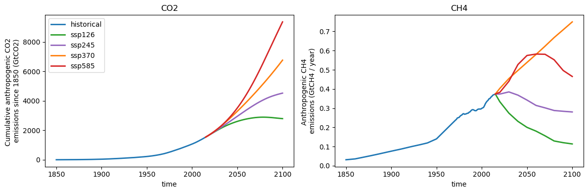
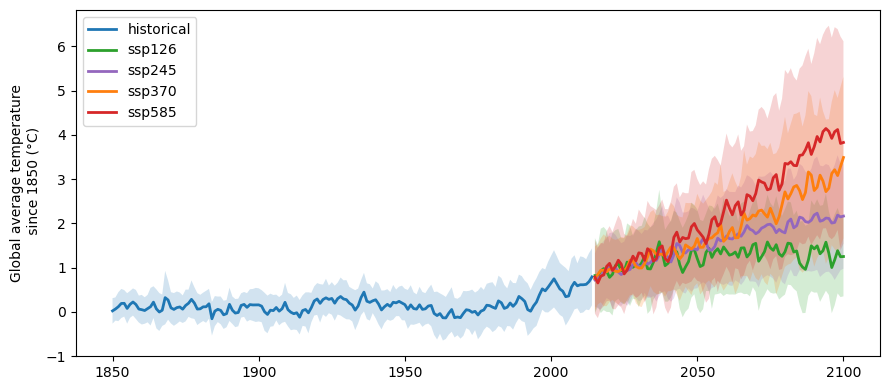
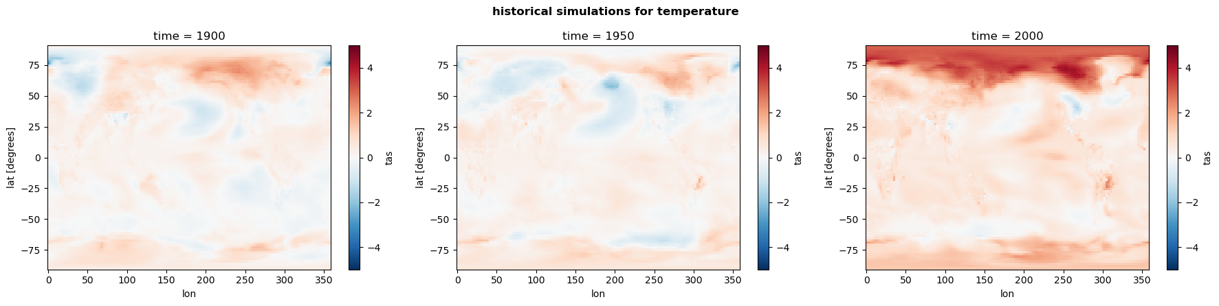
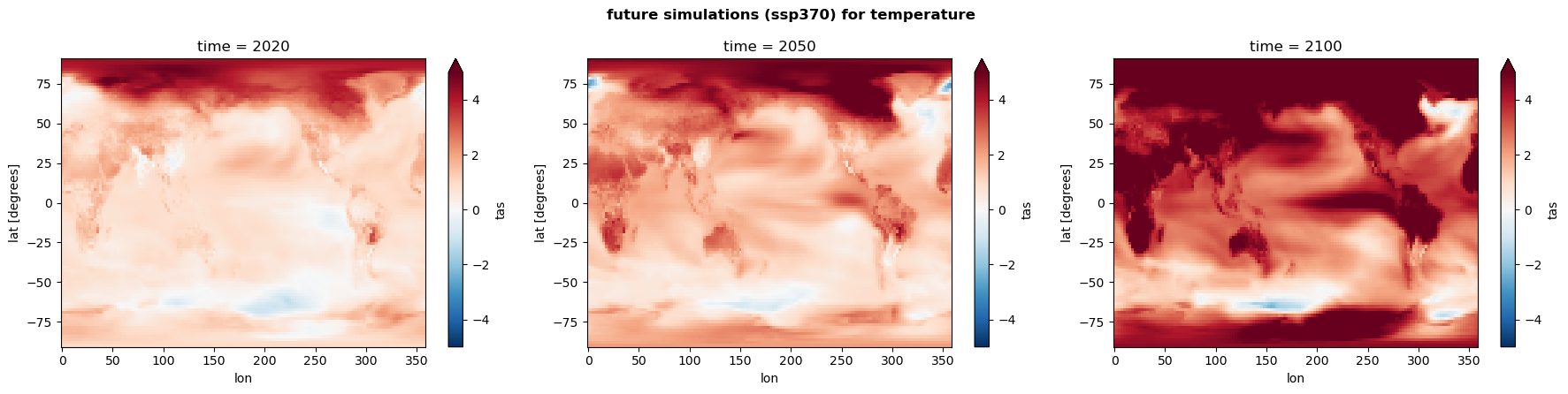
ClimateBench is a spatial-temporal dataset that contains simulations generated by the NorESM2 climate model. It provides both historical simulations & future projections under different scenarios (e.g., ssp245).

Four future scenarios are plotted here: ssp126, ssp245, ssp370, ssp585. These scenarios make different assumptions about future anthropogenic emissions.

def open_dataset(file_path):
    """Flexible opener that can handle both local files (legacy) and cloud urls. IMPORTANT: For this to work the `file_path` must be provided without extension."""
    if 'gs://' in file_path:
        store = f"{file_path}.zarr"
        ds = xr.open_dataset(store, engine='zarr')
    else:
        ds = xr.open_dataset(f"{file_path}.nc")
        # add information to sort and label etc
        ds.attrs['file_name']
    return ds

scenarios = ['historical','ssp126','ssp370','ssp585']
inputs = [os.path.join(train_path , f"inputs_{scenario}") for scenario in scenarios]
inputs.append(os.path.join(test_path, "inputs_ssp245"))
inputs.sort(key=lambda x:x.split('_')[-1])

outputs = [os.path.join(train_path , f"outputs_{scenario}") for scenario in scenarios]
outputs.append(os.path.join(test_path, "outputs_ssp245"))
outputs.sort(key=lambda x:x.split('_')[-1])

fig, axes = plt.subplots(1, 2, figsize=(12,4))
colors  = ['tab:blue','tab:green','tab:purple','tab:orange','tab:red']


for i,input in enumerate(inputs):

    label=input.split('_')[-1]#[:-3]
    X = open_dataset(input)
    x = X.time.data
    
    X['CO2'].plot(label=label,color=colors[i],linewidth=2,ax=axes[0])

    axes[0].set_ylabel("Cumulative anthropogenic CO2 \nemissions since 1850 (GtCO2)")
    
    X['CH4'].plot(label=label,color=colors[i],linewidth=2,ax=axes[1])

    axes[1].set_ylabel("Anthropogenic CH4 \nemissions (GtCH4 / year)")
    
axes[0].set_title('CO2')
axes[1].set_title('CH4')
axes[0].legend()
plt.tight_layout()

../../_images/d8981e9960b56b846f3617fe71b4bdec795c2e1c1a4da7acc7fa8a94f3fe015c.png

fig, ax = plt.subplots(1, 1, figsize=(9,4))

for i,output in enumerate(outputs):

    label=output.split('_')[-1]#[:-3]
    X = open_dataset(output).mean(dim="member")[['tas']].drop_vars(['quantile'])
    x = X.time.data
    
    weights  = np.cos(np.deg2rad(X.lat))
    tas_mean = X['tas'].weighted(weights).mean(['lat', 'lon']).data
    tas_std  = X['tas'].weighted(weights).std(['lat', 'lon']).data
    
    ax.plot(x, tas_mean, label=label,color=colors[i],linewidth=2)
    ax.fill_between(x,tas_mean+tas_std,tas_mean-tas_std,facecolor=colors[i],alpha=0.2)
    
ax.set_ylabel("Global average temperature\n since 1850 (°C)")
ax.legend()
plt.tight_layout()

../../_images/48590e4682e12f06c0a97092b13d60371d5bf09e2bf2432d308e9e09a2cf8586.png

y_his    = open_dataset(os.path.join(train_path , "outputs_historical")).mean(dim="member")[['tas']].drop_vars(['quantile'])
y_ssp370 = open_dataset(os.path.join(train_path,'outputs_ssp370')).mean(dim="member")[['tas']].drop_vars(['quantile'])

fig,axes = plt.subplots(figsize=(18,4.5),ncols=3)
yr0, yr1, yr2 = 1900, 1950, 2000
vmin, vmax = -5, 5

y_his.sel(time=yr0).tas.plot(ax=axes.flat[0],vmin=vmin,vmax=vmax,cmap='RdBu_r')
y_his.sel(time=yr1).tas.plot(ax=axes.flat[1],vmin=vmin,vmax=vmax,cmap='RdBu_r')
y_his.sel(time=yr2).tas.plot(ax=axes.flat[2],vmin=vmin,vmax=vmax,cmap='RdBu_r')

fig.suptitle('historical simulations for temperature',fontweight='bold')
plt.tight_layout()

../../_images/dbd1951983b73e11485813f7a4624dc3a2806c9d424f129f2eb5a831af3ecf3f.png

y_ssp370 = open_dataset(os.path.join(train_path,'outputs_ssp370')).mean(dim="member")[['tas']].drop_vars(['quantile'])


fig,axes = plt.subplots(figsize=(18,4.5),ncols=3)
yr0, yr1, yr2 = 2020, 2050, 2100
vmin, vmax = -5, 5

y_ssp370.sel(time=yr0).tas.plot(ax=axes.flat[0],vmin=vmin,vmax=vmax,cmap='RdBu_r')
y_ssp370.sel(time=yr1).tas.plot(ax=axes.flat[1],vmin=vmin,vmax=vmax,cmap='RdBu_r')
y_ssp370.sel(time=yr2).tas.plot(ax=axes.flat[2],vmin=vmin,vmax=vmax,cmap='RdBu_r')

fig.suptitle('future simulations (ssp370) for temperature',fontweight='bold')
plt.tight_layout()

../../_images/324567e7b762afa9d50967449111f30503e290df64b769149a5d03b21581a2cd.png

y_ssp370 = open_dataset(os.path.join(train_path,'outputs_ssp370')).mean(dim="member")[['tas']].drop_vars(['quantile'])


fig,axes = plt.subplots(figsize=(18,4.5),ncols=3)
yr0, yr1, yr2 = 2020, 2050, 2100
vmin, vmax = -5, 5

y_ssp370.sel(time=yr0).tas.plot(ax=axes.flat[0],vmin=vmin,vmax=vmax,cmap='RdBu_r')
y_ssp370.sel(time=yr1).tas.plot(ax=axes.flat[1],vmin=vmin,vmax=vmax,cmap='RdBu_r')
y_ssp370.sel(time=yr2).tas.plot(ax=axes.flat[2],vmin=vmin,vmax=vmax,cmap='RdBu_r')

fig.suptitle('future simulations (ssp370) for temperature',fontweight='bold')
plt.tight_layout()

Data preprocessing#

We will train the NN using simulations from 3 historical and 3 future scenarios. We will then test the trained NN on the ssp245 scenario.

def prepare_predictor(data_sets, data_path,time_reindex=True):
    """
    Args:
        data_sets list(str): names of datasets
    """
        
    # Create training and testing arrays
    if isinstance(data_sets, str):
        data_sets = [data_sets]
        
    X_all      = []
    length_all = []
    
    for file in data_sets:
        data = open_dataset(f"{data_path}inputs_{file}")
        X_all.append(data)
        length_all.append(len(data.time))
    
    X = xr.concat(X_all,dim='time')
    length_all = np.array(length_all)

    if time_reindex:
        X = X.assign_coords(time=np.arange(len(X.time)))

    return X, length_all
def prepare_predictand(data_sets,data_path,time_reindex=True):
    if isinstance(data_sets, str):
        data_sets = [data_sets]
        
    Y_all = []
    length_all = []
    
    for file in data_sets:
        data = open_dataset(f"{data_path}outputs_{file}")
        Y_all.append(data)
        length_all.append(len(data.time))
    
    length_all = np.array(length_all)
    Y = xr.concat(Y_all,dim='time').mean('member')
    Y = Y.rename({'lon':'longitude','lat': 'latitude'}).transpose('time','latitude', 'longitude').drop_vars(['quantile'])
    if time_reindex:
        Y = Y.assign_coords(time=np.arange(len(Y.time)))
    
    return Y, length_all

# Training set
train_files    = ["historical", "ssp585", "ssp126", "ssp370","hist-aer","hist-GHG"]
X_train_xr, _  = prepare_predictor(train_files,train_path)
y_train_xr, _  = prepare_predictand(train_files,train_path)

# Test set
X_test_xr, _ = prepare_predictor('ssp245', data_path=test_path,time_reindex=False)
y_test_xr, _ = prepare_predictand('ssp245',data_path=test_path,time_reindex=False)

X_train_df = pd.DataFrame({"CO2": X_train_xr["CO2"].data,
                           "CH4": X_train_xr["CH4"].data
                          }, index=X_train_xr["CO2"].coords['time'].data)

X_test_df  = pd.DataFrame({"CO2": X_test_xr["CO2"].data,
                           "CH4": X_test_xr["CH4"].data
                          }, index=X_test_xr["CO2"].coords['time'].data)

y_train_df = y_train_xr["tas"].stack(z=("latitude", "longitude"))
y_train_df = pd.DataFrame(y_train_df.to_pandas())

X_train_df.head()

	CO2	CH4
0	0.188297	0.031306
1	0.377244	0.031742
2	0.573814	0.032178
3	0.778848	0.032614
4	1.020320	0.033049

print(len(y_train_df))
y_train_df.head()

latitude	-90.0										...	90.0
longitude	0.0	2.5	5.0	7.5	10.0	12.5	15.0	17.5	20.0	22.5	...	335.0	337.5	340.0	342.5	345.0	347.5	350.0	352.5	355.0	357.5
time
0	0.320023	0.319946	0.319865	0.319885	0.319860	0.319865	0.319870	0.319911	0.319763	0.319707	...	0.913116	0.913289	0.913116	0.912933	0.912893	0.912659	0.912384	0.912181	0.911825	0.911611
1	-0.667297	-0.667023	-0.667114	-0.667109	-0.667109	-0.667135	-0.667114	-0.667104	-0.667104	-0.666992	...	0.042501	0.042679	0.049225	0.055695	0.055506	0.055227	0.054789	0.054230	0.053604	0.052897
2	-0.058345	-0.058167	-0.058248	-0.058243	-0.058248	-0.058248	-0.058233	-0.058207	-0.058345	-0.058177	...	1.167440	1.167389	1.169657	1.172119	1.172201	1.172190	1.172292	1.172424	1.172709	1.173228
3	0.125870	0.125941	0.125946	0.125941	0.125946	0.125890	0.125951	0.125941	0.125895	0.125982	...	-0.339457	-0.339589	-0.332387	-0.324961	-0.324956	-0.325038	-0.325063	-0.325033	-0.325022	-0.324880
4	0.418304	0.418533	0.418503	0.418523	0.418477	0.418513	0.418503	0.418549	0.418482	0.418564	...	0.577006	0.576996	0.585297	0.593811	0.593740	0.593719	0.593648	0.593801	0.593760	0.593943

5 rows × 13824 columns

Data normalization#

# Standardization
mean, std = X_train_df.mean(), X_train_df.std()

X_train_df   = (X_train_df - mean)/std
X_test_df    = (X_test_df - mean)/std

X_train = X_train_df.to_numpy()
y_train = y_train_df.to_numpy()
X_test = X_test_df.to_numpy()

print(X_train.shape,y_train.shape)

(753, 2) (753, 13824)

Define the neural network structure#

Here we will use a neural network that has 3 hidden layers, and each hidden layer has 64 neurons. The input to the neural network will be the CO2 and CH4 concentrations at each time step.

The neural network outputs are the global surface temperatures (tas), with each neuron of the output layer corresponding to each pixel. There are 13824 pixels in total (96 latitude and 144 longitude).

# set hyperparameters
n_neuron       = 64
activation     = 'relu'
num_epochs     = 50
learning_rate  = 0.001
minibatch_size = 64
model_num      = 1
N_layers       = 3 # number of hidden layers

tf.keras.backend.clear_session()
model = tf.keras.Sequential([
    tf.keras.Input(shape=(X_train.shape[1],)),
    tf.keras.layers.Dense(64, activation="relu",name="hidden_layer_1"),
    tf.keras.layers.Dense(64, activation="relu",name="hidden_layer_2"),
    tf.keras.layers.Dense(64, activation="relu",name="hidden_layer_3"),
    tf.keras.layers.Dense(y_train.shape[1],activation='linear',name="output_layer")
])

model.summary()

Model: "sequential"

┏━━━━━━━━━━━━━━━━━━━━━━━━━━━━━━━━━┳━━━━━━━━━━━━━━━━━━━━━━━━┳━━━━━━━━━━━━━━━┓
┃ Layer (type)                    ┃ Output Shape           ┃       Param # ┃
┡━━━━━━━━━━━━━━━━━━━━━━━━━━━━━━━━━╇━━━━━━━━━━━━━━━━━━━━━━━━╇━━━━━━━━━━━━━━━┩
│ hidden_layer_1 (Dense)          │ (None, 64)             │           192 │
├─────────────────────────────────┼────────────────────────┼───────────────┤
│ hidden_layer_2 (Dense)          │ (None, 64)             │         4,160 │
├─────────────────────────────────┼────────────────────────┼───────────────┤
│ hidden_layer_3 (Dense)          │ (None, 64)             │         4,160 │
├─────────────────────────────────┼────────────────────────┼───────────────┤
│ output_layer (Dense)            │ (None, 13824)          │       898,560 │
└─────────────────────────────────┴────────────────────────┴───────────────┘

 Total params: 907,072 (3.46 MB)

 Trainable params: 907,072 (3.46 MB)

 Non-trainable params: 0 (0.00 B)

model.compile(loss='mse',optimizer=tf.keras.optimizers.Adam(learning_rate=learning_rate))

Train the Neural Network and Save its weights#

early_stop = keras.callbacks.EarlyStopping(monitor='val_loss', patience=20)

history = model.fit(X_train, y_train, 
                    batch_size      = minibatch_size,
                    epochs          = num_epochs,
                    validation_split= 0.2, 
                    verbose         = 1,
                    callbacks       = [early_stop])

Epoch 1/50
10/10 ━━━━━━━━━━━━━━━━━━━━ 1s 59ms/step - loss: 3.6975 - val_loss: 0.5645
Epoch 2/50
10/10 ━━━━━━━━━━━━━━━━━━━━ 0s 45ms/step - loss: 3.4389 - val_loss: 0.5310
Epoch 3/50
10/10 ━━━━━━━━━━━━━━━━━━━━ 0s 45ms/step - loss: 3.1838 - val_loss: 0.4637
Epoch 4/50
10/10 ━━━━━━━━━━━━━━━━━━━━ 0s 45ms/step - loss: 2.1779 - val_loss: 0.3538
Epoch 5/50
10/10 ━━━━━━━━━━━━━━━━━━━━ 0s 39ms/step - loss: 1.2680 - val_loss: 0.2612
Epoch 6/50
10/10 ━━━━━━━━━━━━━━━━━━━━ 0s 46ms/step - loss: 0.7942 - val_loss: 0.2684
Epoch 7/50
10/10 ━━━━━━━━━━━━━━━━━━━━ 0s 39ms/step - loss: 0.4888 - val_loss: 0.2960
Epoch 8/50
10/10 ━━━━━━━━━━━━━━━━━━━━ 0s 47ms/step - loss: 0.4326 - val_loss: 0.2808
Epoch 9/50
10/10 ━━━━━━━━━━━━━━━━━━━━ 1s 55ms/step - loss: 0.3985 - val_loss: 0.2794
Epoch 10/50
10/10 ━━━━━━━━━━━━━━━━━━━━ 0s 45ms/step - loss: 0.3903 - val_loss: 0.2711
Epoch 11/50
10/10 ━━━━━━━━━━━━━━━━━━━━ 0s 39ms/step - loss: 0.3935 - val_loss: 0.2738
Epoch 12/50
10/10 ━━━━━━━━━━━━━━━━━━━━ 0s 45ms/step - loss: 0.3723 - val_loss: 0.2615
Epoch 13/50
10/10 ━━━━━━━━━━━━━━━━━━━━ 0s 44ms/step - loss: 0.3743 - val_loss: 0.2609
Epoch 14/50
10/10 ━━━━━━━━━━━━━━━━━━━━ 0s 39ms/step - loss: 0.3662 - val_loss: 0.2603
Epoch 15/50
10/10 ━━━━━━━━━━━━━━━━━━━━ 0s 46ms/step - loss: 0.3790 - val_loss: 0.2563
Epoch 16/50
10/10 ━━━━━━━━━━━━━━━━━━━━ 0s 39ms/step - loss: 0.3684 - val_loss: 0.2614
Epoch 17/50
10/10 ━━━━━━━━━━━━━━━━━━━━ 0s 45ms/step - loss: 0.3674 - val_loss: 0.2594
Epoch 18/50
10/10 ━━━━━━━━━━━━━━━━━━━━ 0s 44ms/step - loss: 0.3654 - val_loss: 0.2634
Epoch 19/50
10/10 ━━━━━━━━━━━━━━━━━━━━ 0s 45ms/step - loss: 0.3560 - val_loss: 0.2678
Epoch 20/50
10/10 ━━━━━━━━━━━━━━━━━━━━ 0s 46ms/step - loss: 0.3645 - val_loss: 0.2694
Epoch 21/50
10/10 ━━━━━━━━━━━━━━━━━━━━ 0s 48ms/step - loss: 0.3513 - val_loss: 0.2755
Epoch 22/50
10/10 ━━━━━━━━━━━━━━━━━━━━ 0s 45ms/step - loss: 0.3644 - val_loss: 0.2695
Epoch 23/50
10/10 ━━━━━━━━━━━━━━━━━━━━ 0s 45ms/step - loss: 0.3593 - val_loss: 0.2791
Epoch 24/50
10/10 ━━━━━━━━━━━━━━━━━━━━ 0s 39ms/step - loss: 0.3607 - val_loss: 0.2889
Epoch 25/50
10/10 ━━━━━━━━━━━━━━━━━━━━ 0s 45ms/step - loss: 0.3520 - val_loss: 0.2844
Epoch 26/50
10/10 ━━━━━━━━━━━━━━━━━━━━ 0s 39ms/step - loss: 0.3530 - val_loss: 0.2945
Epoch 27/50
10/10 ━━━━━━━━━━━━━━━━━━━━ 0s 46ms/step - loss: 0.3649 - val_loss: 0.2816
Epoch 28/50
10/10 ━━━━━━━━━━━━━━━━━━━━ 0s 45ms/step - loss: 0.3462 - val_loss: 0.2939
Epoch 29/50
10/10 ━━━━━━━━━━━━━━━━━━━━ 0s 46ms/step - loss: 0.3539 - val_loss: 0.2932
Epoch 30/50
10/10 ━━━━━━━━━━━━━━━━━━━━ 0s 45ms/step - loss: 0.3507 - val_loss: 0.2962
Epoch 31/50
10/10 ━━━━━━━━━━━━━━━━━━━━ 0s 46ms/step - loss: 0.3541 - val_loss: 0.3100
Epoch 32/50
10/10 ━━━━━━━━━━━━━━━━━━━━ 1s 53ms/step - loss: 0.3481 - val_loss: 0.3047
Epoch 33/50
10/10 ━━━━━━━━━━━━━━━━━━━━ 0s 39ms/step - loss: 0.3397 - val_loss: 0.3126
Epoch 34/50
10/10 ━━━━━━━━━━━━━━━━━━━━ 0s 45ms/step - loss: 0.3546 - val_loss: 0.3021
Epoch 35/50
10/10 ━━━━━━━━━━━━━━━━━━━━ 0s 45ms/step - loss: 0.3490 - val_loss: 0.3052

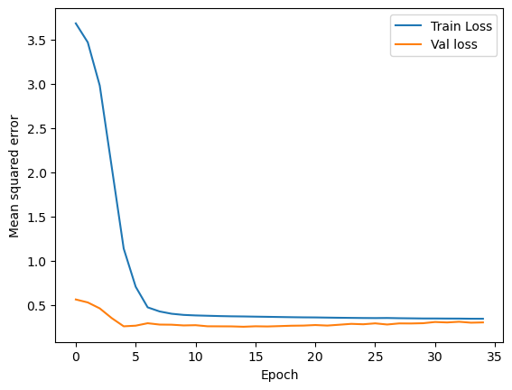
plt.figure()
plt.xlabel('Epoch')
plt.ylabel('Mean squared error')
plt.plot(history.epoch, np.array(history.history['loss']),label='Train Loss')
plt.plot(history.epoch, np.array(history.history['val_loss']),label = 'Val loss')
plt.legend()

<matplotlib.legend.Legend at 0x7e1508e54920>

../../_images/2e2413ba63ea68338bb516d12b51074892077d2d184eb0107611d0087b0ac4ca.png

model_path = os.path.join(cwd,'saved_model')
if os.path.exists(model_path) is False:
    os.makedirs(model_path)

# Save the entire model to a HDF5 file.
# The '.h5' extension indicates that the model should be saved to HDF5.
model.save(os.path.join(model_path,'NN_model.keras'))

Evaluate the trained model#

We will evaluate the trained neural network on the test data set by comparing the neural network predictions against the original surface temperatures simulated under the ssp245 scenario.

# reload the saved model
model = load_model(os.path.join(model_path,'NN_model.keras'))

y_test_pre = model.predict(X_test)
y_test_pre = y_test_pre.reshape(y_test_pre.shape[0], 96, 144)

y_test_pre = xr.Dataset(coords={'time': X_test_xr.time.values, 
                               'latitude': X_test_xr.latitude.values, 
                               'longitude': X_test_xr.longitude.values},
                       data_vars=dict(tas=(['time', 'latitude', 'longitude'], y_test_pre)))

3/3 ━━━━━━━━━━━━━━━━━━━━ 0s 19ms/step

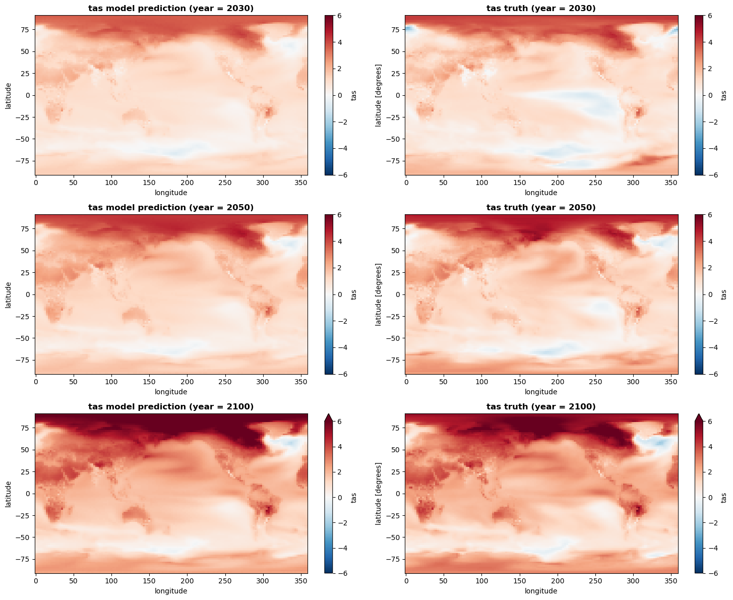
First we check whether the ML model can capture the spatial distribution of global temperatures.

fig, axes = plt.subplots(figsize=(15,12),ncols=2,nrows=3)

yrs = [2030, 2050, 2100]
vmin, vmax    = -6, 6
cmap = 'RdBu_r'
y_test_pre.tas.sel(time=yrs[0]).plot(ax=axes[0,0], vmin=vmin, vmax=vmax,cmap=cmap)
y_test_xr.tas.sel(time=yrs[0]).plot(ax=axes[0,1], vmin=vmin, vmax=vmax,cmap=cmap)

y_test_pre.tas.sel(time=yrs[1]).plot(ax=axes[1,0], vmin=vmin, vmax=vmax,cmap=cmap)
y_test_xr.tas.sel(time=yrs[1]).plot(ax=axes[1,1], vmin=vmin, vmax=vmax,cmap=cmap)

y_test_pre.tas.sel(time=yrs[2]).plot(ax=axes[2,0], vmin=vmin, vmax=vmax,cmap=cmap)
y_test_xr.tas.sel(time=yrs[2]).plot(ax=axes[2,1], vmin=vmin, vmax=vmax,cmap=cmap)


for i, ax in enumerate(axes.flat):
    # left column: model prediction
    if i % 2 == 0:
        ax.set_title(f'tas model prediction (year = {yrs[i//2]})',fontweight='bold')
    # right column: truth tas from ssp245 simulations
    else:
        ax.set_title(f'tas truth (year = {yrs[i//2]})',fontweight='bold')
plt.tight_layout()

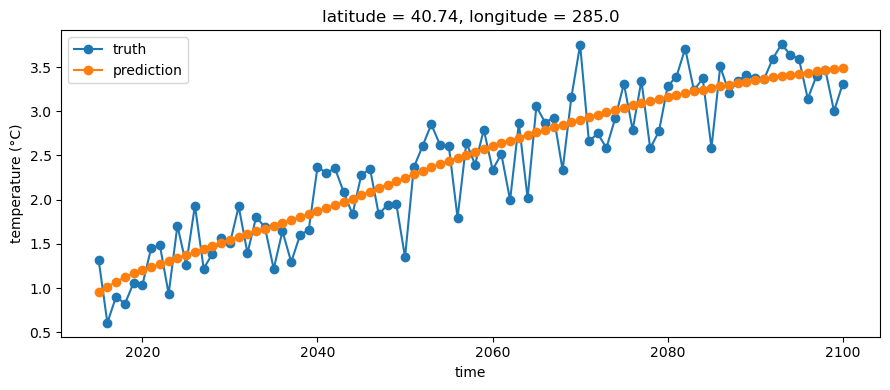
../../_images/27c1fa8319925862fe92b373aa723fd8cbf0ef3fdcfd259d82a8fb064a4ab608.png

Then we will also check how well the ML model can reproduce the time series of a given location. Here we will take NYC as an example (40.7128° N, 74.0060° W)

lat = 40.7128
lon = -74.0060%360

fig,ax = plt.subplots(figsize=(9,4))
y_test_xr.sel(latitude=lat,longitude=lon,method='nearest').tas.plot(marker='o',ax=ax,label='truth')
y_test_pre.sel(latitude=lat,longitude=lon,method='nearest').tas.plot(marker='o',ax=ax,label='prediction')

ax.legend()
ax.set_ylabel('temperature (°C)')

plt.tight_layout()

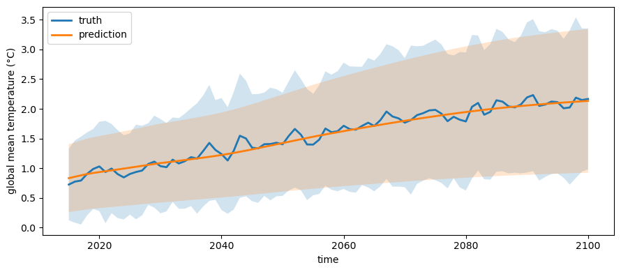
../../_images/9111353f1b762c8cfb7efac5fde2ca850c017cbde4c8a76a3b78f5c33853a3e9.png

Finally, we will check whether the ML model can capture the time series of global average temperature

def global_mean_std_plot(X,label,color,ax,var='tas'):
    weights  = np.cos(np.deg2rad(X.latitude))
    tas_mean = X[var].weighted(weights).mean(['latitude', 'longitude']).data
    tas_std  = X[var].weighted(weights).std(['latitude', 'longitude']).data
    
    x = X.time.data

    ax.plot(x, tas_mean, label=label,color=color,linewidth=2)
    ax.fill_between(x,tas_mean+tas_std,tas_mean-tas_std,facecolor=color,alpha=0.2)

fig,ax = plt.subplots(figsize=(9,4))

global_mean_std_plot(y_test_xr,label='truth',ax=ax,color='tab:blue')
global_mean_std_plot(y_test_pre,label='prediction',ax=ax,color='tab:orange')

ax.set_xlabel('time')
ax.set_ylabel('global mean temperature (°C)')
ax.legend()
plt.tight_layout()

../../_images/0e8316302a406632b3347915aedf1b9d42eea3cbe374c56a9c955138f92fcd2a.png

Train a CNN to predict the global temperature map#

Next, we will look at using a CNN rather than a NN to predict the global temperature map. This example is based on the notebook by Weiwei Zhan and Francesco Immorlano.

We start with preparing the datasets as before.

X_train_df = pd.DataFrame({"CO2": X_train_xr["CO2"].data,
                           "CH4": X_train_xr["CH4"].data
                          }, index=X_train_xr["CO2"].coords['time'].data)

X_test_df  = pd.DataFrame({"CO2": X_test_xr["CO2"].data,
                           "CH4": X_test_xr["CH4"].data
                          }, index=X_test_xr["CO2"].coords['time'].data)

y_train = y_train_xr['tas'].data
y_test  = y_test_xr['tas'].data

For the CNN, the predictant (target) will be a 2-D map of global temperature, rather than a 1-D array (as it was for the NN)

Data Normalization#

Let’s normalize the input predictors by their mean and standard deviation.

	# Standardization
mean, std = X_train_df.mean(), X_train_df.std()

X_train_df   = (X_train_df - mean)/std
X_test_df    = (X_test_df - mean)/std

X_train = X_train_df.to_numpy()
X_test = X_test_df.to_numpy()

print(X_train.shape,y_train.shape,X_test.shape,y_test.shape)

(753, 2) (753, 96, 144) (86, 2) (86, 96, 144)

Define the CNN architecture#

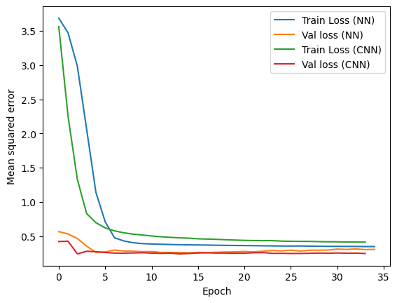
The CNN architecture used here consists of several upsampling blocks.

We set the dimensions of the hidden layers (i.e., number of neurons) in order to reach the size of the target maps (96x144) in a proportional way (in particular by doubling the dimensions in each upsampling block) through the various upsampling blocks.

Here are the hyperparameters for the CNN training. Note that these hyperparameters here are for demonstration purposes only and they are not optimized.

n_filters  = 32  # number of filters
n_neurons  = 32  # number of neurons in the Dense layer
activation     = 'relu' # activation function
kernel_size    = 4
learning_rate  = 0.001
minibatch_size = 64
num_epochs     = 100

model = Sequential()


model.add(Input(shape=(X_train.shape[1],))),
model.add(Dense(n_filters*12*18, input_shape=(X_train.shape[1],), activation=activation)) # shape: (6912,1)
model.add(Reshape((12,18,n_filters))) # shape: (12,18,32)

# Upsample to 24x36
model.add(Conv2DTranspose(filters=n_filters, kernel_size=kernel_size, 
                          activation=activation, strides=2, padding='same')) # shape: (24,36,32)

# Upsample to 48x72
model.add(Conv2DTranspose(filters=n_filters, kernel_size=kernel_size, 
                          activation=activation, strides=2, padding='same')) # shape: (48,72,32)

# Upsample to 96x144
model.add(Conv2DTranspose(filters=n_filters, kernel_size=kernel_size, 
                          activation=activation, strides=2, padding='same')) # shape: (96,144,32)

model.add(Conv2DTranspose(filters=1, kernel_size=kernel_size, activation="linear", padding="same")) # shape: (96,144,1)


model.summary()
model.compile(loss='mse',optimizer=tf.keras.optimizers.Adam(learning_rate=learning_rate))

/srv/conda/envs/notebook/lib/python3.12/site-packages/keras/src/layers/core/dense.py:93: UserWarning: Do not pass an `input_shape`/`input_dim` argument to a layer. When using Sequential models, prefer using an `Input(shape)` object as the first layer in the model instead.
  super().__init__(activity_regularizer=activity_regularizer, **kwargs)

Model: "sequential_1"

┏━━━━━━━━━━━━━━━━━━━━━━━━━━━━━━━━━┳━━━━━━━━━━━━━━━━━━━━━━━━┳━━━━━━━━━━━━━━━┓
┃ Layer (type)                    ┃ Output Shape           ┃       Param # ┃
┡━━━━━━━━━━━━━━━━━━━━━━━━━━━━━━━━━╇━━━━━━━━━━━━━━━━━━━━━━━━╇━━━━━━━━━━━━━━━┩
│ dense (Dense)                   │ (None, 6912)           │        20,736 │
├─────────────────────────────────┼────────────────────────┼───────────────┤
│ reshape (Reshape)               │ (None, 12, 18, 32)     │             0 │
├─────────────────────────────────┼────────────────────────┼───────────────┤
│ conv2d_transpose                │ (None, 24, 36, 32)     │        16,416 │
│ (Conv2DTranspose)               │                        │               │
├─────────────────────────────────┼────────────────────────┼───────────────┤
│ conv2d_transpose_1              │ (None, 48, 72, 32)     │        16,416 │
│ (Conv2DTranspose)               │                        │               │
├─────────────────────────────────┼────────────────────────┼───────────────┤
│ conv2d_transpose_2              │ (None, 96, 144, 32)    │        16,416 │
│ (Conv2DTranspose)               │                        │               │
├─────────────────────────────────┼────────────────────────┼───────────────┤
│ conv2d_transpose_3              │ (None, 96, 144, 1)     │           513 │
│ (Conv2DTranspose)               │                        │               │
└─────────────────────────────────┴────────────────────────┴───────────────┘

 Total params: 70,497 (275.38 KB)

 Trainable params: 70,497 (275.38 KB)

 Non-trainable params: 0 (0.00 B)

Train and save the CNN model#

early_stop = keras.callbacks.EarlyStopping(monitor='val_loss', patience=20)


history_cnn = model.fit(X_train, y_train, 
                    batch_size      = minibatch_size,
                    epochs          = num_epochs,
                    validation_split= 0.2, 
                    verbose         = 1,
                    callbacks       = [early_stop])

Epoch 1/100
10/10 ━━━━━━━━━━━━━━━━━━━━ 13s 1s/step - loss: 3.7040 - val_loss: 0.4203
Epoch 2/100
10/10 ━━━━━━━━━━━━━━━━━━━━ 12s 1s/step - loss: 2.4507 - val_loss: 0.4251
Epoch 3/100
10/10 ━━━━━━━━━━━━━━━━━━━━ 12s 1s/step - loss: 1.4679 - val_loss: 0.2405
Epoch 4/100
10/10 ━━━━━━━━━━━━━━━━━━━━ 12s 1s/step - loss: 0.8678 - val_loss: 0.2778
Epoch 5/100
10/10 ━━━━━━━━━━━━━━━━━━━━ 12s 1s/step - loss: 0.7540 - val_loss: 0.2717
Epoch 6/100
10/10 ━━━━━━━━━━━━━━━━━━━━ 12s 1s/step - loss: 0.6219 - val_loss: 0.2596
Epoch 7/100
10/10 ━━━━━━━━━━━━━━━━━━━━ 12s 1s/step - loss: 0.5837 - val_loss: 0.2516
Epoch 8/100
10/10 ━━━━━━━━━━━━━━━━━━━━ 13s 1s/step - loss: 0.5377 - val_loss: 0.2496
Epoch 9/100
10/10 ━━━━━━━━━━━━━━━━━━━━ 12s 1s/step - loss: 0.5442 - val_loss: 0.2529
Epoch 10/100
10/10 ━━━━━━━━━━━━━━━━━━━━ 12s 1s/step - loss: 0.5319 - val_loss: 0.2565
Epoch 11/100
10/10 ━━━━━━━━━━━━━━━━━━━━ 12s 1s/step - loss: 0.5203 - val_loss: 0.2510
Epoch 12/100
10/10 ━━━━━━━━━━━━━━━━━━━━ 12s 1s/step - loss: 0.4994 - val_loss: 0.2475
Epoch 13/100
10/10 ━━━━━━━━━━━━━━━━━━━━ 12s 1s/step - loss: 0.4962 - val_loss: 0.2502
Epoch 14/100
10/10 ━━━━━━━━━━━━━━━━━━━━ 12s 1s/step - loss: 0.4874 - val_loss: 0.2403
Epoch 15/100
10/10 ━━━━━━━━━━━━━━━━━━━━ 12s 1s/step - loss: 0.4691 - val_loss: 0.2455
Epoch 16/100
10/10 ━━━━━━━━━━━━━━━━━━━━ 12s 1s/step - loss: 0.4537 - val_loss: 0.2526
Epoch 17/100
10/10 ━━━━━━━━━━━━━━━━━━━━ 12s 1s/step - loss: 0.4417 - val_loss: 0.2551
Epoch 18/100
10/10 ━━━━━━━━━━━━━━━━━━━━ 13s 1s/step - loss: 0.4483 - val_loss: 0.2515
Epoch 19/100
10/10 ━━━━━━━━━━━━━━━━━━━━ 12s 1s/step - loss: 0.4518 - val_loss: 0.2515
Epoch 20/100
10/10 ━━━━━━━━━━━━━━━━━━━━ 12s 1s/step - loss: 0.4640 - val_loss: 0.2486
Epoch 21/100
10/10 ━━━━━━━━━━━━━━━━━━━━ 12s 1s/step - loss: 0.4363 - val_loss: 0.2502
Epoch 22/100
10/10 ━━━━━━━━━━━━━━━━━━━━ 12s 1s/step - loss: 0.4265 - val_loss: 0.2566
Epoch 23/100
10/10 ━━━━━━━━━━━━━━━━━━━━ 12s 1s/step - loss: 0.4361 - val_loss: 0.2582
Epoch 24/100
10/10 ━━━━━━━━━━━━━━━━━━━━ 12s 1s/step - loss: 0.4562 - val_loss: 0.2474
Epoch 25/100
10/10 ━━━━━━━━━━━━━━━━━━━━ 12s 1s/step - loss: 0.4086 - val_loss: 0.2481
Epoch 26/100
10/10 ━━━━━━━━━━━━━━━━━━━━ 12s 1s/step - loss: 0.4247 - val_loss: 0.2457
Epoch 27/100
10/10 ━━━━━━━━━━━━━━━━━━━━ 12s 1s/step - loss: 0.4361 - val_loss: 0.2460
Epoch 28/100
10/10 ━━━━━━━━━━━━━━━━━━━━ 13s 1s/step - loss: 0.4165 - val_loss: 0.2485
Epoch 29/100
10/10 ━━━━━━━━━━━━━━━━━━━━ 12s 1s/step - loss: 0.4222 - val_loss: 0.2516
Epoch 30/100
10/10 ━━━━━━━━━━━━━━━━━━━━ 12s 1s/step - loss: 0.4176 - val_loss: 0.2497
Epoch 31/100
10/10 ━━━━━━━━━━━━━━━━━━━━ 12s 1s/step - loss: 0.4059 - val_loss: 0.2530
Epoch 32/100
10/10 ━━━━━━━━━━━━━━━━━━━━ 12s 1s/step - loss: 0.4235 - val_loss: 0.2493
Epoch 33/100
10/10 ━━━━━━━━━━━━━━━━━━━━ 12s 1s/step - loss: 0.4106 - val_loss: 0.2509
Epoch 34/100
10/10 ━━━━━━━━━━━━━━━━━━━━ 12s 1s/step - loss: 0.3990 - val_loss: 0.2452

plt.figure()
plt.xlabel('Epoch')
plt.ylabel('Mean squared error')
plt.plot(history.epoch, np.array(history.history['loss']),label='Train Loss (NN)')
plt.plot(history.epoch, np.array(history.history['val_loss']),label = 'Val loss (NN)')
plt.plot(history_cnn.epoch, np.array(history_cnn.history['loss']),label='Train Loss (CNN)')
plt.plot(history_cnn.epoch, np.array(history_cnn.history['val_loss']),label = 'Val loss (CNN)')
plt.legend()

<matplotlib.legend.Legend at 0x7e143eba8860>

../../_images/27ddb490f1d23fd2fa70e50ffcc9ccedf0a38f5ac100748024e6e65b4539bd96.png

# Save the entire model to a HDF5 file.
# The '.h5' extension indicates that the model should be saved to HDF5.
model.save(os.path.join(model_path,'CNN_model.keras'))

Evaluate the trained model#

We will load the model since it takes a while to train.

# reload the saved model
model = load_model(os.path.join(model_path,'CNN_model.keras'))

y_test_pre = model.predict(X_test)
y_test_pre = y_test_pre.reshape(y_test_pre.shape[0], 96, 144)
y_test_pre = xr.Dataset(coords={'time': X_test_xr.time.values, 
                               'latitude': X_test_xr.latitude.values, 
                               'longitude': X_test_xr.longitude.values},
                       data_vars=dict(tas=(['time', 'latitude', 'longitude'], y_test_pre)))

3/3 ━━━━━━━━━━━━━━━━━━━━ 1s 405ms/step

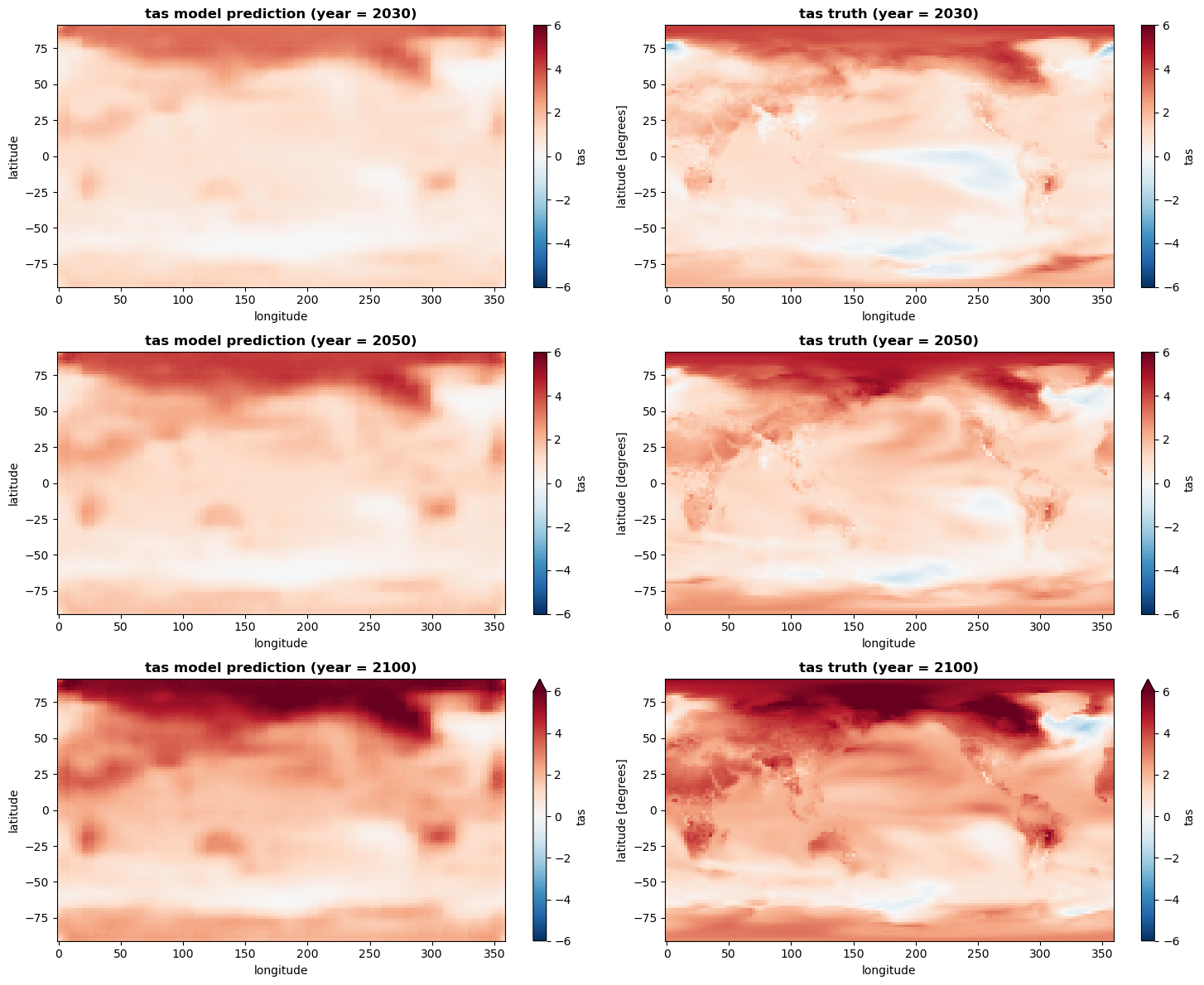
First we check whether the ML model can capture the spatial distribution of global temperature

fig, axes = plt.subplots(figsize=(15,12),ncols=2,nrows=3)

yrs = [2030, 2050, 2100]
vmin, vmax    = -6, 6
cmap = 'RdBu_r'
y_test_pre.tas.sel(time=yrs[0]).plot(ax=axes[0,0], vmin=vmin, vmax=vmax,cmap=cmap)
y_test_xr.tas.sel(time=yrs[0]).plot(ax=axes[0,1], vmin=vmin, vmax=vmax,cmap=cmap)

y_test_pre.tas.sel(time=yrs[1]).plot(ax=axes[1,0], vmin=vmin, vmax=vmax,cmap=cmap)
y_test_xr.tas.sel(time=yrs[1]).plot(ax=axes[1,1], vmin=vmin, vmax=vmax,cmap=cmap)

y_test_pre.tas.sel(time=yrs[2]).plot(ax=axes[2,0], vmin=vmin, vmax=vmax,cmap=cmap)
y_test_xr.tas.sel(time=yrs[2]).plot(ax=axes[2,1], vmin=vmin, vmax=vmax,cmap=cmap)


for i, ax in enumerate(axes.flat):
    # left column: model prediction
    if i % 2 == 0:
        ax.set_title(f'tas model prediction (year = {yrs[i//2]})',fontweight='bold')
    # right column: truth tas from ssp245 simulations
    else:
        ax.set_title(f'tas truth (year = {yrs[i//2]})',fontweight='bold')
plt.tight_layout()

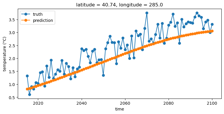
../../_images/bedbdd2921495ae371a7aa8c8f7f983402b87e3aaec2a041b27739646e3bdba6.png

Then we also check whether the ML model can reproduce the time series of a given location. Here we take NYC as an example (40.7128° N, 74.0060° W)

lat = 40.7128
lon = -74.0060%360

fig,ax = plt.subplots(figsize=(9,4))
y_test_xr.sel(latitude=lat,longitude=lon,method='nearest').tas.plot(marker='o',ax=ax,label='truth')
y_test_pre.sel(latitude=lat,longitude=lon,method='nearest').tas.plot(marker='o',ax=ax,label='prediction')

ax.legend()
ax.set_ylabel('temperature (°C)')

Text(0, 0.5, 'temperature (°C)')

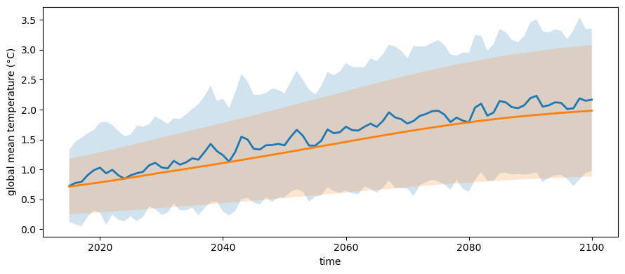
../../_images/4caa3d7360d627bf0494331e8c0922b6c3747629c9e9573e90edbb5f030a79a6.png

Finally we will check whether the ML model can capture the time series of global average temperatures.

def global_mean_std_plot(X,label,color,ax,var='tas'):
    weights  = np.cos(np.deg2rad(X.latitude))
    tas_mean = X[var].weighted(weights).mean(['latitude', 'longitude']).data
    tas_std  = X[var].weighted(weights).std(['latitude', 'longitude']).data
    
    x = X.time.data

    ax.plot(x, tas_mean, label=label,color=color,linewidth=2)
    ax.fill_between(x,tas_mean+tas_std,tas_mean-tas_std,facecolor=color,alpha=0.2)

fig,ax = plt.subplots(figsize=(9,4))

global_mean_std_plot(y_test_xr,label='truth',ax=ax,color='tab:blue')
global_mean_std_plot(y_test_pre,label='prediction',ax=ax,color='tab:orange')

ax.set_xlabel('time')
ax.set_ylabel('global mean temperature (°C)')
plt.tight_layout()

../../_images/01f2fa1fd82a3ed18f0bef963d24126f8bcbac028d50cee9dbc60cd003c5c3fd.png

Try it yourself#

Set the random seed. These models randomly initialize their weights (and SGD samples random batches), so results shift slightly run to run. Add tf.random.set_seed(42) before building each model and confirm the losses reproduce.
Test on a different scenario. Retrain on the other scenarios and test on ssp585 instead of ssp245. Does the emulator do worse when it has to extrapolate to a hotter scenario than any it trained on, rather than interpolate?
Tune the CNN. Try a larger kernel_size, more n_filters, or more up-sampling blocks. Can you sharpen the blurry maps without overfitting the small dataset?
Add a metric. Pass metrics=['RootMeanSquaredError'] to model.compile and watch the RMSE (in °C) alongside the MSE loss during training.

The last two run in seconds and neither retrains a model, so they are good to try in class if there is time.

Read off the architecture, no training. Rebuild only the CNN Sequential(...) block with a different kernel_size (try 3 and 8) or a different n_filters, then call model.summary(). Do not call model.fit. The output stays 96 by 144 whatever the kernel size: why? (Look at padding='same' and the three stride-2 up-sampling layers.) How does the total parameter count change as you enlarge the kernel or add filters, and does it stay well below the dense NN’s roughly 907,000?
Which data augmentations suit a climate map? The lecture introduced data augmentation (rotations, flips, translations, resizing) as a way to expand an image dataset when you do not have enough of it. For a global surface-temperature map on a latitude/longitude grid, which of these give a physically plausible new training example and which do not? Think about flipping the map north to south (swapping the hemispheres), rolling it in longitude (shifting the prime meridian), or rotating it 90 degrees (mixing latitude with longitude). No code required, just reason it through.

Tutorial on Global Temperature Trends with Deep Learning

Contents

Tutorial on Global Temperature Trends with Deep Learning#

Predicting global temperature from greenhouse gas concentrations#

Visualization of the ClimateBench Data#

Data preprocessing#

Data normalization#

Define the neural network structure#

Train the Neural Network and Save its weights#

Evaluate the trained model#

Train a CNN to predict the global temperature map#

Data Normalization#

Define the CNN architecture#

Train and save the CNN model#

Evaluate the trained model#

Try it yourself#