Introduction to Artificial Neural Networks

Deep learning is where much of the recent innovation in machine learning for climate science and environmental sustainability is happening. In this section we will:

• Define the artificial neural network (ANN) and see how it generalizes the linear models we’ve already met.

• Understand activation functions and where the non-linearity of a neural network comes from.

• Walk through the steps and best practices to build a neural network in practice.

• Know the main hyperparameters that define a network’s architecture and the ones that control its training.

• Discuss applications of neural networks to climate model parameterizations and tuning.

The figures in the first part of this page are all generated from data with a few lines of numpy and scikit-learn’s built-in multilayer perceptron, so you can see each idea rather than take it on faith.

import numpy as np
import matplotlib.pyplot as plt
import warnings
from sklearn.neural_network import MLPRegressor, MLPClassifier
from sklearn.linear_model import LinearRegression
from sklearn.preprocessing import StandardScaler
from sklearn.model_selection import train_test_split
from sklearn.datasets import make_moons
from sklearn.metrics import r2_score, log_loss

warnings.filterwarnings("ignore")   # silence sklearn convergence chatter for a clean page
np.random.seed(0)

From biological to artificial neural networks

The conceptual roots of the neural network were recognized by the 2024 Nobel Prize in Physics, awarded to John Hopfield and Geoffrey Hinton. Hopfield introduced the Hopfield network (1982), a simple recurrent network that can store and recall patterns, drawing on ideas from statistical physics. Hinton and collaborators introduced the Boltzmann machine, a stochastic neural network in which nodes make probabilistic decisions about being on or off. Both were foundational ideas that led to what we now call the artificial neural network.

The name comes from a loose analogy with the brain. A biological neuron accumulates a membrane potential and, once it crosses a threshold, “fires” — the synapse activates. An artificial neural network mimics this with activation functions that introduce non-linearities between layers. The biological version is far more complicated, but even this simple analogy is enough to build a system that can learn essentially any non-linear function.

The perceptron and the fully connected layer

The simplest neural network is the perceptron. We take some inputs, multiply them by weights, and apply a step-function activation: negative values map to 0, positive values map to 1, producing a single output. This was a forerunner of the modern neural network.

Instead of a single output, we can connect the inputs to a whole layer of outputs — a fully connected layer. Each input connects to every unit in the next layer through a learned weight, and an activation function is applied. Written out, a layer looks very much like linear regression:

\[ \text{output} = \phi\left( W\,\mathbf{x} + \mathbf{b} \right) \]

where \(\mathbf{x}\) is the input vector, \(W\) is the weight matrix, \(\mathbf{b}\) is the bias vector (the intercept), and \(\phi\) is the activation function. The only thing that distinguishes this from linear regression is the non-linear \(\phi\) applied to the weighted sum.

From a layer to a Multilayer Perceptron

Stacking fully connected layers gives a Multilayer Perceptron (MLP), also called a feedforward neural network. With a single hidden layer, the input features \(x_1, x_2, \ldots\) (there could be a hundred of them) are combined by a learned weight matrix, passed through an activation to produce a hidden layer, and then combined again to produce the output:

\[ \text{Hidden} = \phi_{\text{bottom}}\left( W_{\text{bottom}}\,\text{Input} + \mathbf{b}_{\text{bottom}} \right) \]

\[ \text{Output} = \phi_{\text{top}}\left( W_{\text{top}}\,\text{Hidden} + \mathbf{b}_{\text{top}} \right) \]

A useful rule of thumb for depth:

• 1 layer ≈ logistic regression (with a step/logistic activation),

• 2 layers = a shallow neural network,

• 3 or more layers = deep learning.

The hidden layers hold hidden variables — higher-dimensional features the network learns for the specific problem. Unlike linear regression, where a weight multiplying “temperature” or “precipitation” has a direct interpretation, these hidden features are hard to read off directly. This is why neural networks are often described as black boxes: the input-to-output mapping passes through many non-linear activations and becomes difficult to interpret. Explainable-AI (XAI) techniques exist to probe why a network produces the mapping it does, but interpretability remains a genuine trade-off for the flexibility neural networks buy us.

Activation functions — where the non-linearity arises

Activation functions are the “magic” of neural networks: they are where the non-linearity comes from. Without them, a stack of linear layers — even hundreds of them — could be rewritten as a single linear transformation, and the network could not represent non-linear functions.

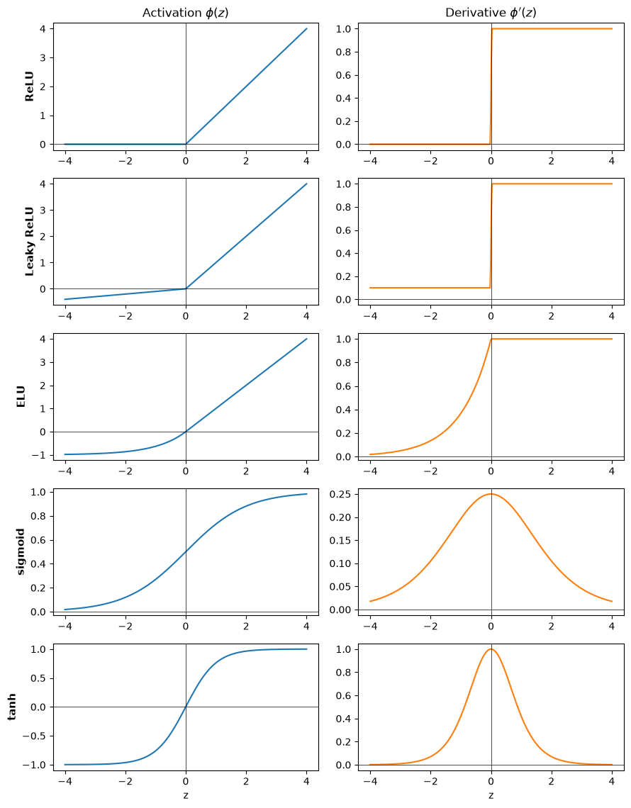
Each row below shows one activation function (left) alongside its derivative (right). ReLU zeros out negatives and keeps positives unchanged (note its abrupt, stepwise derivative). Sigmoid and tanh squash their inputs into a bounded range with smooth derivatives — useful when you want to constrain an output to a known physical range. Leaky ReLU and ELU keep a small response for negative inputs to preserve gradient flow.

z = np.linspace(-4, 4, 400)

def relu(z):         return np.maximum(0.0, z)
def leaky(z, a=0.1): return np.where(z > 0, z, a * z)
def elu(z, a=1.0):   return np.where(z > 0, z, a * (np.exp(z) - 1))
sigmoid = 1.0 / (1.0 + np.exp(-z))
tanh    = np.tanh(z)

funcs = {"ReLU": relu(z), "Leaky ReLU": leaky(z), "ELU": elu(z),
         "sigmoid": sigmoid, "tanh": tanh}

# one row per activation: function on the left, its derivative on the right
fig, axes = plt.subplots(len(funcs), 2, figsize=(9, 2.3 * len(funcs)))
for row, (name, yv) in enumerate(funcs.items()):
    axL, axR = axes[row]
    axL.plot(z, yv, color="C0")
    axR.plot(z, np.gradient(yv, z), color="C1")
    axL.set_ylabel(name, fontsize=11, fontweight="bold")
    for ax in (axL, axR):
        ax.axhline(0, color="k", lw=0.5); ax.axvline(0, color="k", lw=0.5)
    if row == 0:
        axL.set_title(r"Activation $\phi(z)$"); axR.set_title(r"Derivative $\phi'(z)$")
    if row == len(funcs) - 1:
        axL.set_xlabel("z"); axR.set_xlabel("z")
plt.tight_layout(); plt.show()

Neural networks as universal approximators

One of the real powers of neural networks is that they are universal function approximators. The Universal Approximation Theorem (Cybenko & Hornik, 1989; Leshno et al., 1993) says that by making a network wide enough (enough weights per layer) or deep enough (enough layers), it can represent any continuous function.

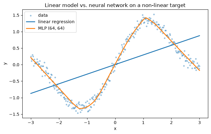
This goes beyond linear functions. Linear regression (even polynomial regression) learns weights that scale the inputs in a way we can write down. A neural network can approximate genuinely non-linear functions. Below we fit both a linear regression and an MLP to the same non-linear, noisy target. The linear model can only draw a straight line; the MLP follows the curve. The printed \(R^2\) scores make the difference concrete (higher is better; a straight line through curved data scores poorly).

# A non-linear 1-D target with a little noise
X = np.linspace(-3, 3, 300).reshape(-1, 1)
y = np.sin(1.5 * X).ravel() + 0.3 * X.ravel() + 0.1 * np.random.randn(X.shape[0])

Xs = StandardScaler().fit_transform(X)                    # scale inputs for the MLP
linear = LinearRegression().fit(X, y)
mlp = MLPRegressor(hidden_layer_sizes=(64, 64), activation="relu",
                   max_iter=4000, random_state=0).fit(Xs, y)

y_lin, y_mlp = linear.predict(X), mlp.predict(Xs)
print(f"Linear regression R^2 : {r2_score(y, y_lin):.3f}")
print(f"MLP (64, 64)      R^2 : {r2_score(y, y_mlp):.3f}")

plt.figure(figsize=(7, 4.5))
plt.scatter(X, y, s=8, alpha=0.35, label="data")
plt.plot(X, y_lin, lw=2, label="linear regression")
plt.plot(X, y_mlp, lw=2, label="MLP (64, 64)")
plt.title("Linear model vs. neural network on a non-linear target")
plt.xlabel("x"); plt.ylabel("y"); plt.legend(); plt.tight_layout(); plt.show()

Linear regression R^2 : 0.349
MLP (64, 64)      R^2 : 0.984

Wide enough to approximate

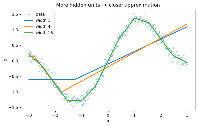
“Wide enough” is also an important point. The same target is fit below by MLPs with a single hidden layer of increasing width. A network with only a couple of hidden units can bend the line a little; adding units lets it track the curve ever more closely, with the \(R^2\) climbing accordingly.

widths = [1, 4, 16]
plt.figure(figsize=(7, 4.5))
plt.scatter(X, y, s=8, alpha=0.3, label="data")
for w in widths:
    m = MLPRegressor(hidden_layer_sizes=(w,), activation="relu", solver="lbfgs",
                     max_iter=8000, random_state=0).fit(Xs, y)
    print(f"hidden width {w:2d}: R^2 = {r2_score(y, m.predict(Xs)):.3f}")
    plt.plot(X, m.predict(Xs), lw=2, label=f"width {w}")
plt.title("More hidden units -> closer approximation")
plt.xlabel("x"); plt.ylabel("y"); plt.legend(); plt.tight_layout(); plt.show()

hidden width  1: R^2 = 0.434
hidden width  4: R^2 = 0.515

hidden width 16: R^2 = 0.988

Learning the weights: backpropagation

The parameters a network must learn are the weight matrices and bias vectors of every layer — and there can be very many of them. A deep network can have hundreds of thousands of weights.

Training uses backpropagation:

1. Forward pass. With the current weights, propagate the inputs through the layers (applying weights and activations) to produce predictions.

2. Loss. Evaluate a loss function comparing predictions to targets.

3. Backward pass. Compute the gradient of the loss with respect to every weight, and take a step that reduces the loss.

Gradients are computed by automatic differentiation, which applies the chain rule sequentially over the network’s computational graph to get exact gradients.

A key difficulty is the exploding / vanishing gradient problem: repeated multiplication by large (or small) factors through the chain rule can make weights unstable, so the loss oscillates or diverges (exploding), or stops updating (vanishing). This is especially challenging for deep networks. Many remedies exist — gradient clipping, careful weight initialization, smaller learning rates, batch normalization, residual connections, and the choice of activation function.

The loss landscape and the learning rate

The learning rate tells gradient descent how far to move the weights at each step. We can see why it matters on a problem simple enough to draw: fitting a line \(y = w\,x + b\) by minimizing mean squared error gives a bowl-shaped loss surface over the two parameters \((w, b)\). Gradient descent walks downhill toward the minimum. The three paths below start from the same point with different learning rates.

# Toy linear data; the MSE of a line y = w*x + b is a bowl over the two parameters
xd = np.random.randn(80)
yd = 2.0 * xd + 1.0 + 0.3 * np.random.randn(80)

def mse(w, b):
    p = w * xd + b
    return np.mean((p - yd) ** 2)

def grad(w, b):
    p = w * xd + b
    return 2 * np.mean((p - yd) * xd), 2 * np.mean(p - yd)

# evaluate the loss surface on a grid of (w, b)
ws = np.linspace(-1, 5, 200); bs = np.linspace(-2, 4, 200)
WW, BB = np.meshgrid(ws, bs)
ZZ = np.array([[mse(w, b) for w in ws] for b in bs])

def descend(lr, steps=40, start=(-0.5, -1.5)):
    w, b = start; path = [(w, b)]; loss = [mse(w, b)]
    for _ in range(steps):
        gw, gb = grad(w, b); w -= lr * gw; b -= lr * gb
        path.append((w, b)); loss.append(mse(w, b))
    return np.array(path), np.array(loss)

rates = {"too small (0.02)": 0.02, "well chosen (0.3)": 0.3, "too large (1.02)": 1.02}

fig, (axL, axR) = plt.subplots(1, 2, figsize=(12, 5))
cf = axL.contourf(WW, BB, ZZ, levels=30, cmap="viridis")
fig.colorbar(cf, ax=axL, label="MSE loss")
axL.contour(WW, BB, ZZ, levels=8, colors="white", alpha=0.3, linewidths=0.5)
for label, lr in rates.items():
    path, loss = descend(lr)
    axL.plot(path[:, 0], path[:, 1], marker="o", ms=3, lw=1.3, label=label)
    axR.plot(loss, marker="o", ms=3, lw=1.3, label=label)
    print(f"{label:20s} -> final (w, b) = ({path[-1,0]:8.2f}, {path[-1,1]:8.2f}), "
          f"final loss = {loss[-1]:.2e}")
print("(true parameters used to generate the data: w = 2.0, b = 1.0)")
axL.scatter([2.0], [1.0], c="red", marker="*", s=220, zorder=5, label="minimum")
axL.set(title="Loss surface with gradient-descent paths", xlabel="w (slope)",
        ylabel="b (intercept)", xlim=(-1, 5), ylim=(-2, 4))
axL.legend(fontsize=8, loc="upper right")
axR.set(title="Loss vs. iteration", xlabel="iteration", ylabel="MSE loss (log scale)",
        yscale="log")
axR.legend(fontsize=8)
plt.tight_layout(); plt.show()

too small (0.02)     -> final (w, b) = (    1.16,     0.30), final loss = 9.91e-01
well chosen (0.3)    -> final (w, b) = (    2.06,     0.99), final loss = 8.70e-02
too large (1.02)     -> final (w, b) = ( 3920.90, -6692.61), final loss = 6.65e+07
(true parameters used to generate the data: w = 2.0, b = 1.0)

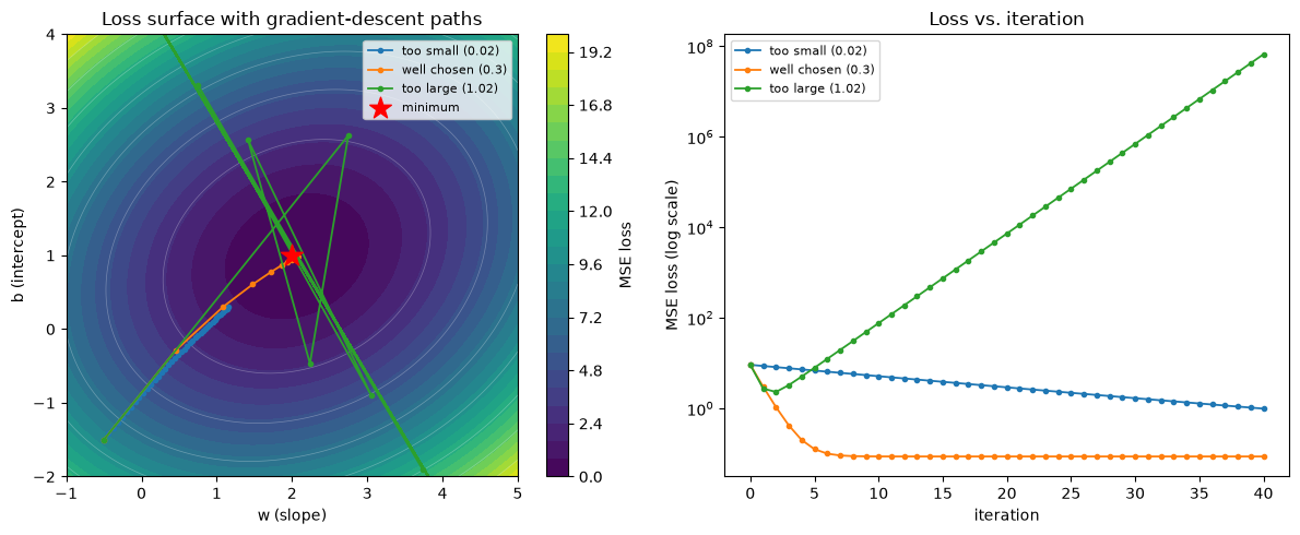
The colored surface on the left is the bowl-shaped loss (darker = lower), with its minimum at the true \((w, b) = (2, 1)\) marked by a star. Three gradient-descent runs start from the same lower-left corner. With too small a learning rate the point crawls and barely leaves the corner in the budget of steps; with a well-chosen rate it descends straight to the minimum; with too large a rate the steps overshoot and shoot out of the frame — the loss diverges. The right panel shows the same three runs as loss versus iteration (log scale): the well-chosen rate drops steeply toward zero, the too-small rate decreases but stalls far above it, and the too-large rate climbs as it diverges. Real networks have millions of parameters, so this landscape is vastly higher-dimensional, but the intuition carries over.

Building a neural network in practice

The workflow parallels what we discussed earlier in the course for supervised and unsupervised learning, with more knobs to turn:

1. Define the problem — classification vs. regression — which fixes the loss function (e.g., mean squared error for regression; binary/categorical cross-entropy for classification; mean absolute error or Huber as alternatives). One real constraint: because training differentiates the loss, the loss must be differentiable.

2. Pre-process the data — training/validation/test split, and normalization / scaling of the inputs. As with linear or logistic regression, well-scaled inputs make it much easier and faster to find optimal weights.

3. Choose the architecture and implement it in a deep-learning library.

For real deep learning we use TensorFlow with the Keras front end, or PyTorch — libraries that provide automatic differentiation and GPU support. (An API, Application Programming Interface, is simply a way for programs to communicate; Keras is a high-level API for defining networks layer by layer.) For the small illustrations on this page scikit-learn’s MLPClassifier / MLPRegressor are enough; for the assignments and larger climate problems you’ll use Keras.

Epochs, batches, and monitoring training

We rarely train on the whole dataset at once. Stochastic gradient descent uses a random batch of the data at each step; one epoch is a full pass through the training set. Training over multiple epochs, on batches, tends to find a more generalizable solution — and is often a practical necessity, since image or climate datasets can be far too large to fit in memory.

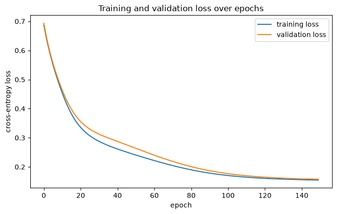
We watch the training loss and a held-out validation loss fall over epochs. Below we train a small classifier on the two-moons dataset and record both after each epoch. The validation loss tracks the training loss and sits slightly above it — the expected, healthy pattern. If the validation loss instead started to rise while the training loss kept falling, that would signal overfitting, and early stopping would halt training at the turn.

Xm, ym = make_moons(n_samples=1000, noise=0.25, random_state=0)
Xtr, Xval, ytr, yval = train_test_split(Xm, ym, test_size=0.3, random_state=0)
sc = StandardScaler().fit(Xtr); Xtr, Xval = sc.transform(Xtr), sc.transform(Xval)

clf = MLPClassifier(hidden_layer_sizes=(32, 32), activation="relu",
                    max_iter=1, warm_start=True, random_state=0)
train_loss, val_loss = [], []
for epoch in range(150):
    clf.partial_fit(Xtr, ytr, classes=[0, 1])
    train_loss.append(log_loss(ytr, clf.predict_proba(Xtr), labels=[0, 1]))
    val_loss.append(log_loss(yval, clf.predict_proba(Xval), labels=[0, 1]))

print(f"final training loss   : {train_loss[-1]:.3f}")
print(f"final validation loss : {val_loss[-1]:.3f}")
print(f"validation accuracy   : {clf.score(Xval, yval):.3f}")

plt.figure(figsize=(7, 4.5))
plt.plot(train_loss, label="training loss")
plt.plot(val_loss, label="validation loss")
plt.title("Training and validation loss over epochs")
plt.xlabel("epoch"); plt.ylabel("cross-entropy loss"); plt.legend()
plt.tight_layout(); plt.show()

final training loss   : 0.154
final validation loss : 0.158
validation accuracy   : 0.933

What overfitting looks like

The run above generalizes well. To see overfitting, we make the problem hard for the model to memorize and generalize at once: shrink the training set, add a lot of noise, and use a much larger network with almost no regularization. Now watch the two losses part ways.

Xo, yo = make_moons(n_samples=120, noise=0.45, random_state=0)
Xtr2, Xval2, ytr2, yval2 = train_test_split(Xo, yo, test_size=0.4, random_state=0)
sc2 = StandardScaler().fit(Xtr2); Xtr2, Xval2 = sc2.transform(Xtr2), sc2.transform(Xval2)

over = MLPClassifier(hidden_layer_sizes=(200, 200), activation="relu", alpha=1e-6,
                     max_iter=1, warm_start=True, random_state=0)
tr_loss, va_loss = [], []
for epoch in range(400):
    over.partial_fit(Xtr2, ytr2, classes=[0, 1])
    tr_loss.append(log_loss(ytr2, over.predict_proba(Xtr2), labels=[0, 1]))
    va_loss.append(log_loss(yval2, over.predict_proba(Xval2), labels=[0, 1]))

best = int(np.argmin(va_loss))
print(f"validation loss is lowest at epoch {best} (loss {va_loss[best]:.3f})")
print(f"final training loss   : {tr_loss[-1]:.3f}")
print(f"final validation loss : {va_loss[-1]:.3f}  <- much higher than at its minimum")

plt.figure(figsize=(7, 4.5))
plt.plot(tr_loss, label="training loss")
plt.plot(va_loss, label="validation loss")
plt.axvline(best, color="gray", ls="--", label=f"early-stopping point (epoch {best})")
plt.title("Overfitting: validation loss turns back up")
plt.xlabel("epoch"); plt.ylabel("cross-entropy loss"); plt.legend()
plt.tight_layout(); plt.show()

validation loss is lowest at epoch 26 (loss 0.386)
final training loss   : 0.145
final validation loss : 0.973  <- much higher than at its minimum

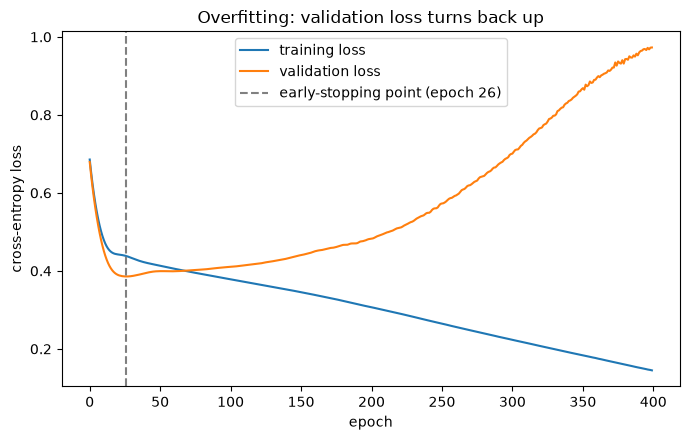
This is the pattern the healthy run only hinted at. The training loss keeps falling toward zero as the oversized network memorizes the noisy training points, but the validation loss bottoms out and then climbs — past that point the model is fitting noise, not signal, so it generalizes worse. Early stopping ends training at the dashed line (the validation minimum), keeping the most generalizable model. More training data and regularization (L1/L2, dropout — below) are the other standard remedies.

Architecture and training hyperparameters

Neural networks expose many more choices than the scikit-learn algorithms we’ve used: the number of hidden layers, the number of neurons per layer, and the activation at each layer and at the output. Rules of thumb: keep layer sizes near a power of two to avoid bottlenecks, change sizes gradually, and use a softmax output for classification. Beyond these heuristics, architecture design is “more art than science.”

On the training side, the key knobs are the learning rate (illustrated above), the loss function (MSE / MAE / Huber for regression; cross-entropy for classification), the optimizer, and the batch size. Optimizers are all variants of stochastic gradient descent (SGD): plain SGD; SGD with momentum (adds a velocity term); AdaGrad / AdaDelta / RMSprop (adapt the learning rate during training); and Adam (Adaptive Moment Estimation), which combines RMSprop and momentum and is one of the most widely used optimizers in practice.

Avoiding overfitting through regularization

Because networks have so many weights, they can overfit. Regularization helps: L1 / L2 regularization penalizes the weights in the loss (L2 discourages large weights; L1 encourages sparsity); batch normalization rescales a layer’s inputs using batch statistics; and dropout randomly removes weights during training, which reduces effective capacity — and, applied at inference, is also used to add an uncertainty estimate to a network that would otherwise output a single value.

---

Neural Networks in Climate and Environmental Science

A recurring question in this field is: how can we emulate a complex, non-linear, high-dimensional environmental process with machine learning? Two applications below — emulating sub-grid parameterizations and tuning climate-model parameters — put the universal-approximation property to work.

Emulating sub-grid processes (parameterizations)

A climate model divides the Earth — atmosphere, ocean, land, at many vertical levels — into a 3-D grid and steps the environmental variables forward in time. Because climate projections run for hundreds of years, the models must be computationally efficient, so grid boxes are large — a typical grid spacing is ~25–100 km.

Everything happening at scales smaller than a grid box — shallow and deep convection, cloud microphysics, the radiative effects of clouds — still affects the grid-box averages of temperature, humidity, and so on. These sub-grid effects are represented by parameterizations: simplified models of the aggregated effect of small-scale processes within a grid box over a time step.

A concrete example is super-parameterization. A standard atmosphere model such as CAM5 uses conventional parameterizations at ~100 km spacing. SPCAM5 instead embeds a much higher-resolution atmospheric model inside each grid box — far more accurate, but so computationally expensive it cannot be used for routine long-term climate runs. The machine-learning idea is to train a neural network on SPCAM5 to reproduce its sub-grid behavior, then drop that network back into the coarse model in place of the parameterization. Because a network’s inference is fast, the emulator delivers close to SPCAM5 quality at a small fraction of the cost. One of the first papers to demonstrate deep learning for sub-grid processes (published in 2018) used exactly this setup, with super-parameterized CAM as the ground truth.

A practical obstacle is software: many climate models are written in Fortran — hundreds of thousands of lines of legacy code — while the machine-learning libraries are in Python. Coupling the two is genuinely hard; groups bridge Fortran and Python, rewrite parts of the model in Python, or rebuild the model in a language like Julia where these optimization approaches can be expressed directly.

Tuning climate-model parameters

Neural networks can also improve a climate model without replacing its parameterizations — by helping tune its parameters. Parameterizations contain many parameters whose values start from physical understanding but are then tuned so the model better matches large-scale observations (for example the entrainment rate of convective clouds, or the fall velocity of ice crystals, which sets how long-lived clouds are).

Doing this by hand is slow. A perturbed-parameter ensemble (PPE) runs the climate model many times — say ~500 runs spanning ~40 atmospheric parameters. Because each run is expensive, only a limited number of parameter sets can be sampled directly. A neural network then learns the non-linear mapping from input parameters to model outputs, acting as a cheap surrogate for the full model. With that surrogate we can explore far more of the parameter space, study how parameters interact non-linearly, and identify which parameters the model is most sensitive to — which also flags where a process may be poorly represented physically.

Parametric vs. structural error

Tuning often reveals that no parameter set fits all the observations well. That points to structural error rather than parametric error:

• Parametric error — the equations are right but a parameter value is wrong. If a model is \(y = w_1 x\) and \(w_1\) is off, tuning \(w_1\) fixes it.

• Structural error — the equations themselves are wrong (the truth is really \(x^2\), not \(x\)). No amount of tuning the existing parameters can recover the observations.

Parametric errors are what tuning and PPE surrogates address. Structural errors send us back to improve the underlying parameterizations. Either way, these tools progressively point to where a model can be improved.