Autoencoders, VAEs, and Latent Representations

The third state-of-the-art generative architecture, after the GAN and the diffusion model, is the variational autoencoder (VAE). It grows out of dimensionality reduction, so this page also closes a loop begun in the unsupervised learning unit. We will:

• Review dimensionality reduction and place deep learning methods among the linear ones.

• Build an autoencoder: a neural network that learns a low dimensional representation of its own input.

• See what a latent space buys us: denoising, generation, semi-supervised learning, anomaly detection.

• Define the variational autoencoder and why its latent space is smoother.

• Survey scientific uses of latent representations, including convective organization.

Dimensionality reduction, revisited

Dimensionality reduction techniques reduce the number of features in a dataset while retaining the essential information, for visualization, analysis, feature engineering, or model performance. Data often live on a lower dimensional manifold: however many variables we record, the system has limited degrees of freedom, and only so many states actually occur. The main method families:

• Projection methods transform the data linearly to lower dimensions: principal component analysis (PCA), which for spatio-temporal climate data goes by the name empirical orthogonal function (EOF) analysis.

• Manifold learning methods capture nonlinear structure (t-SNE, UMAP, etc.).

• Deep learning methods transform the data nonlinearly using a neural network: autoencoders and variational autoencoders, this section’s subject.

Recall what PCA does: it finds the directions of greatest variance and projects onto them. Here is the digits dataset (1797 images of handwritten digits, 8 by 8 pixels, so 64 features) projected onto its first two principal components.

import numpy as np
import matplotlib.pyplot as plt
from sklearn.datasets import load_digits
from sklearn.decomposition import PCA

rng = np.random.default_rng(0)

digits = load_digits()
Xd = digits.data / 16.0          # scale pixel values to [0, 1]
yd = digits.target

pca2 = PCA(n_components=2).fit(Xd)
Zp = pca2.transform(Xd)

plt.figure(figsize=(6, 5))
sc = plt.scatter(Zp[:, 0], Zp[:, 1], c=yd, cmap="tab10", s=8, alpha=0.7)
plt.colorbar(sc, label="digit")
plt.xlabel("first principal component"); plt.ylabel("second principal component")
plt.title("Digits in 2-D: PCA")
plt.tight_layout(); plt.show()

print(f"variance explained by 2 components: {pca2.explained_variance_ratio_.sum():.2f}")

variance explained by 2 components: 0.29

Two linear components separate a few digits (0s and 6s hold together) but most classes overlap heavily, and they capture under a third of the variance. A linear projection is simply not flexible enough for images. That is the opening for a neural network.

Autoencoders

An autoencoder is nonlinear dimensionality reduction with neural networks. It has two halves:

• An encoder network takes the input (here 64 pixels) and compresses it through progressively narrower layers down to a small bottleneck, the latent representation: here just 2 numbers.

• A decoder network takes the latent representation and tries to reconstruct the original input from it.

The two are trained together as one network whose training target is its own input: a supervised learning setup where the loss is the reconstruction error. The bottleneck is what makes it interesting: to reconstruct 64 pixels from 2 numbers, the network must discover what actually varies across the dataset. Unlike PCA, the encoding is not restricted to directions of greatest variance or to linear maps; it is whatever nonlinear representation the data support. Either half can be any architecture we have seen (dense, CNN for images, RNN for sequences), chosen to match the input type.

We can build one with MLPRegressor by making the target equal to the input and giving the hidden layers an hourglass shape, 64 to 2 to 64.

from sklearn.neural_network import MLPRegressor

ae = MLPRegressor(hidden_layer_sizes=(64, 2, 64), activation="tanh",
                  max_iter=2000, tol=1e-6, random_state=0)
ae.fit(Xd, Xd)                    # the target IS the input

def encode(X):
    "run the first two layers of the trained network"
    h = np.tanh(X @ ae.coefs_[0] + ae.intercepts_[0])
    return np.tanh(h @ ae.coefs_[1] + ae.intercepts_[1])

def decode(Z):
    "run the last two layers of the trained network"
    h = np.tanh(Z @ ae.coefs_[2] + ae.intercepts_[2])
    return np.clip(h @ ae.coefs_[3] + ae.intercepts_[3], 0, 1)

Z = encode(Xd)
recon_ae = decode(Z)
recon_pca = pca2.inverse_transform(Zp)

mse_ae = ((recon_ae - Xd) ** 2).mean()
mse_pca = ((recon_pca - Xd) ** 2).mean()
print(f"reconstruction MSE through a 2-D bottleneck:")
print(f"  autoencoder: {mse_ae:.4f}")
print(f"  PCA:         {mse_pca:.4f}")

reconstruction MSE through a 2-D bottleneck:
  autoencoder: 0.0326
  PCA:         0.0524

Squeezed through the same 2 number bottleneck, the autoencoder reconstructs the images with clearly lower error than PCA: the nonlinearity is doing real work. Seeing the reconstructions makes the comparison tangible.

fig, axes = plt.subplots(3, 8, figsize=(9, 4))
show = rng.choice(len(Xd), 8, replace=False)
for col, i in enumerate(show):
    for row, (img, label) in enumerate([(Xd[i], "original"),
                                        (recon_ae[i], "autoencoder"),
                                        (recon_pca[i], "PCA")]):
        ax = axes[row, col]
        ax.imshow(img.reshape(8, 8), cmap="gray_r", vmin=0, vmax=1)
        ax.set_xticks([]); ax.set_yticks([])
        if col == 0:
            ax.set_ylabel(label, fontsize=9)
fig.suptitle("Reconstruction through a 2-D bottleneck")
plt.tight_layout(); plt.show()

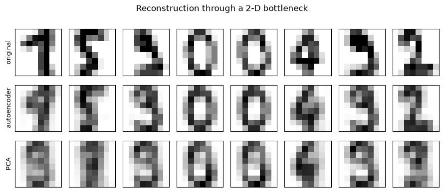
Both reconstructions are blurry (2 numbers cannot hold 64 pixels of detail), but the autoencoder’s outputs are recognizable digits far more often than PCA’s. Now look at where the encoder puts each image in its 2-D latent space, side by side with the PCA projection.

fig, axes = plt.subplots(1, 2, figsize=(11, 4.5), sharey=False)
for ax, (Zi, name) in zip(axes, [(Zp, "PCA"), (Z, "autoencoder latent space")]):
    sc = ax.scatter(Zi[:, 0], Zi[:, 1], c=yd, cmap="tab10", s=8, alpha=0.7)
    ax.set_title(name)
fig.colorbar(sc, ax=axes, label="digit")
plt.show()

The autoencoder was never told the labels, yet its latent space groups the digit classes into more distinct clumps than PCA manages. Images that are similar sit near each other, which is exactly what makes latent spaces useful: clustering, similarity search, and the applications below all run on this geometry.

Denoising

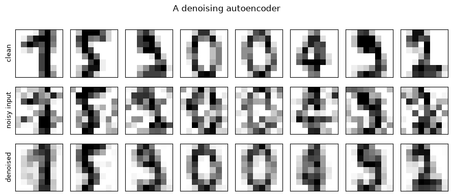
Because the bottleneck keeps only the most representative structure in the data, an autoencoder can be turned into a noise remover. The clean recipe is the denoising autoencoder: corrupt each training input with random noise, but keep the clean image as the training target. The network then cannot succeed by memorizing pixels; it must learn what digits look like underneath the noise. (Simply round-tripping noisy images through the 2-D autoencoder above does not work: its reconstructions are too coarse to beat the noise pixel for pixel, so here we allow the bottleneck 16 dimensions.)

X_noisy_train = np.clip(Xd + 0.30 * rng.standard_normal(Xd.shape), 0, 1)
dae = MLPRegressor(hidden_layer_sizes=(64, 16, 64), activation="tanh",
                   max_iter=2000, tol=1e-6, random_state=0)
dae.fit(X_noisy_train, Xd)          # noisy input, CLEAN target

X_noisy = np.clip(Xd + 0.30 * rng.standard_normal(Xd.shape), 0, 1)  # fresh noise
denoised = np.clip(dae.predict(X_noisy), 0, 1)

fig, axes = plt.subplots(3, 8, figsize=(9, 4))
for col, i in enumerate(show):
    for row, (img, label) in enumerate([(Xd[i], "clean"),
                                        (X_noisy[i], "noisy input"),
                                        (denoised[i], "denoised")]):
        ax = axes[row, col]
        ax.imshow(img.reshape(8, 8), cmap="gray_r", vmin=0, vmax=1)
        ax.set_xticks([]); ax.set_yticks([])
        if col == 0:
            ax.set_ylabel(label, fontsize=9)
fig.suptitle("A denoising autoencoder")
plt.tight_layout(); plt.show()

print(f"MSE to the clean image, noisy input:     {((X_noisy - Xd) ** 2).mean():.4f}")
print(f"MSE to the clean image, denoised output: {((denoised - Xd) ** 2).mean():.4f}")

MSE to the clean image, noisy input:     0.0517
MSE to the clean image, denoised output: 0.0205

The denoised output is more than twice as close to the clean image as the noisy input it was given, on noise the network never saw during training. The same trick, predicting the clean signal from a corrupted version of it, is also the training objective at the heart of the diffusion models on the previous page.

Generating new samples

The decoder does not care whether its input came from the encoder. Feed it any point in the latent space and it will render an image. Sweeping a grid across the latent space maps out the latent manifold: what the model believes the data look like everywhere in its coordinate system.

g1 = np.linspace(*np.percentile(Z[:, 0], [2, 98]), 8)
g2 = np.linspace(*np.percentile(Z[:, 1], [2, 98]), 8)
step = 8 + 2                       # 8 pixel tiles, 2 blank pixels between them
canvas = np.zeros((8 * step - 2, 8 * step - 2))
for r, z2 in enumerate(g2[::-1]):
    for c, z1 in enumerate(g1):
        img = decode(np.array([[z1, z2]]))[0].reshape(8, 8)
        canvas[r * step:r * step + 8, c * step:c * step + 8] = img

plt.figure(figsize=(6, 6))
plt.imshow(canvas, cmap="gray_r")
plt.xticks([]); plt.yticks([])
plt.xlabel("latent dimension 1"); plt.ylabel("latent dimension 2")
plt.title("Decoding a grid of latent points: the latent manifold")
plt.tight_layout(); plt.show()

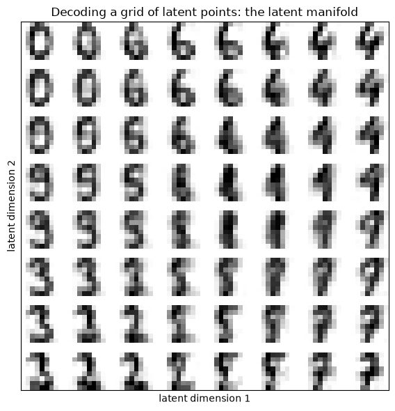
Every tile is a generated image: none of these exact digits exists in the training set. Neighboring tiles morph smoothly into one another, and the clusters from the scatter plot reappear as regions of the grid that render similar digits. But notice the seams: between clusters the decoder produces smeared shapes that are not convincing digits. The plain autoencoder’s latent space has holes, regions no training image maps to, where the decoder was never supervised. That weakness is what the variational autoencoder fixes.

Semi-supervised learning

Latent spaces also help when labels are scarce, a constant condition in environmental science, where labeling means expert time. Suppose we could afford to label only 50 of the 1797 digit images. We can still encode all of them, then classify unlabeled images by which labeled ones they sit near in latent space.

from sklearn.neighbors import KNeighborsClassifier

rng_lab = np.random.default_rng(42)
labeled = rng_lab.choice(len(yd), 50, replace=False)
mask = np.ones(len(yd), bool)
mask[labeled] = False

for name, F in [("64 raw pixels", Xd), ("2-D PCA", Zp), ("2-D latent", Z)]:
    knn = KNeighborsClassifier(n_neighbors=3).fit(F[labeled], yd[labeled])
    acc = knn.score(F[mask], yd[mask])
    print(f"3-NN with 50 labels on {name:13s}: {acc:.1%} accuracy on the rest")

3-NN with 50 labels on 64 raw pixels: 75.4% accuracy on the rest
3-NN with 50 labels on 2-D PCA      : 51.1% accuracy on the rest
3-NN with 50 labels on 2-D latent   : 74.0% accuracy on the rest

With the same 50 labels, nearest neighbors in the autoencoder’s 2 dimensions (about 74 percent accuracy) classify far better than in PCA’s 2 dimensions (about 51 percent), and nearly match all 64 raw pixels (about 75 percent). Two learned numbers per image retain most of what the 64 pixels know about digit identity. (A fourth use, anomaly detection, follows the same logic as on the previous page: points that land far from everything else in latent space are candidates for contamination, instrument error, or genuinely unusual events.)

Variational autoencoders

The variational autoencoder keeps the encoder-bottleneck-decoder shape but makes the encoding probabilistic. Instead of mapping an input to a single latent point, the encoder outputs the parameters of a distribution (a mean and a variance per latent dimension). During training a latent point is sampled from that distribution, with random noise added, and the decoder must reconstruct the input from the perturbed sample. The loss adds a second term to the reconstruction error: the KL divergence between the encoder’s distribution and a standard Gaussian, which measures how far the learned latent distribution strays from the Gaussian prior. Minimizing it pulls the cloud of latent points toward a smooth Gaussian ball.

The effect is exactly what the latent manifold above was missing: the latent space is smoothed out, with no holes, because every neighborhood gets covered by some training sample’s noise. Sampling any point from the Gaussian prior and decoding it yields a plausible new sample, which is what makes the VAE a genuinely generative model, effectively learning the underlying distribution of the data rather than a fixed mapping. Classic VAE visualizations of clothing images (Fashion-MNIST) show shirts, dresses, and pants occupying their own regions of latent space, with interpolations between them rendering plausible intermediate garments.

Latent representations for scientific analysis

In science the samples we care about are not digits but fields and observations, and the latent space becomes an instrument for analysis.

Classifying convection in climate model output. Work by Mooers and collaborators encoded large volumes of climate model vertical velocity profiles (snapshots of updraft structure through the atmospheric column) with an encoder. Different regions of the resulting latent space correspond to physically distinct regimes: shallow convection, midlatitude storm tracks, deep convection. The latent space turns an unmanageable volume of model output into a map on which regimes can be identified and counted.

Ice crystals in climate models. Ice-containing clouds strongly impact climate, but they are hard to model because ice crystals take enormously diverse habits (shapes). Recent work uses self-supervised learning to learn latent representations of crystal morphology from ice crystal imagery: a vision transformer pre-trained on many cloud particle images learns robust representations without hand labels, which can then be used for science driven tasks such as quantifying ice crystal diversity, improving the characterization of ice crystals and helping constrain their role in Earth’s climate system.

Learning convective organization. Climate models must parameterize convection inside grid boxes 25 to 100 km across, and their known precipitation biases (raining too little and too often, missing the extremes) trace partly to ignoring how organized sub-grid convection is. Shamekh, Lamb, Huang, and Gentine (PNAS, 2023) trained a VAE on high resolution precipitable water fields from global storm resolving simulations, jointly with a network predicting precipitation at the next time step from large scale variables plus the VAE’s four latent “org” variables. The org informed network recovers the full precipitation distribution, extremes included. A PCA of the latent variables finds that a single direction explains about 98 percent of their variance, and decoding along it (the latent manifold trick from the digits example) shows it measures sub-grid convective organization: an interpretable, autocorrelated quantity a climate model could carry and evolve.

Summary

• Autoencoders learn nonlinear low dimensional representations by reconstructing their own input through a bottleneck; they beat PCA at equal dimensionality and enable denoising, generation, semi-supervised learning, and anomaly detection.

• Variational autoencoders make the encoding probabilistic and regularize the latent space toward a Gaussian, closing the holes that break generation from a plain autoencoder.

• Latent representations are scientific instruments: they classify convection regimes, organize ice crystal morphology, and discover an interpretable, predictable convective organization parameter that improves precipitation extremes.

This closes the generative modeling arc: uncertainty and how to score it, GANs and diffusion models, and the VAE with its latent spaces.