Tutorial: Generative Models for Single-Particle Aerosol Measurements

This hands-on tutorial accompanies the notes on generative modeling, GANs and diffusion models, and VAEs. We put all three architectures to work on the same real instrument data set and ask three different questions of it.

The data come from the Single Particle Soot Photometer (SP2), a specialized research instrument used to measure aerosols (small particulate matter) during airborne research field campaigns. Aerosol particles that strongly absorb light, such as black carbon (also known as soot) and some mineral dusts and iron oxide particles, can have important effects on climate. Quantifying the mass of these aerosols in the atmosphere is important for understanding the role they play in warming the atmosphere locally. The SP2 has traditionally been used to measure black carbon, the most important absorbing aerosol in terms of its effects on climate, but it can also detect other types of aerosol particle such as mineral dust and iron oxides.

This tutorial uses real data sets from several recent research papers. Here the SP2 was used to measure laboratory proxies of seven types of aerosol that the instrument can detect. The SP2 detects an aerosol by sending it through a strong laser beam, which heats an absorbing particle until it incandesces, that is, until it burns up in the beam. What the SP2 measures is the light signal from each particle as it burns up. Different types of aerosol burn differently because they have different physicochemical properties. The challenge is to work out how these particles can be told apart from their time series: 400 points, corresponding to a signal 80 microseconds long.

During airborne field campaigns we would have no labels, unlike these laboratory proxies, where we know what we are measuring. So in this tutorial we explore several approaches using generative machine learning to differentiate different types of aerosols using the SP2 time series alone.

The laboratory data set was introduced by Lamb (2019), Classification of iron oxide aerosols by a single particle soot photometer using supervised machine learning, which classified these same aerosols with a random forest, the supervised counterpart to what we do here, and the method from the supervised learning unit. The version of the data we use, and the VAE analysis this tutorial adapts, are from Doshi and Lamb (2025), Unsupervised classification of absorbing aerosols with the SP2 via a variational autoencoder. Both were published in Atmospheric Measurement Techniques. Because the signals were measured in the laboratory for seven known aerosol types, we have ground-truth labels to check our unsupervised results against. The 2025 paper’s own code (in PyTorch, using the pyroVED library) is at github.com/kdlamb/SP2-VAE; everything here is written from scratch in TensorFlow/Keras.

Conventional SP2 analysis reduces each trace to a couple of scalar features (peak height, peak position, color ratio). The question is whether unsupervised deep learning can pull more out of the full signal shape.

The three examples:

1. VAE: compress each signal to two numbers and look at where the seven aerosol types land in that latent space.

2. GAN: train a generator on fullerene soot only, then use it as an anomaly detector that flags everything that is not fullerene soot.

3. Conditional diffusion model: learn to generate a realistic SP2 signal on demand for any of the seven classes.

The VAE and the GAN train in well under a minute on a laptop CPU; the diffusion model takes about eight. Each one seeds itself, so the three examples are independent and you can re-run any of them on its own.

Setup

Everything below uses TensorFlow/Keras, NumPy, matplotlib, scikit-learn (for the evaluation metrics only) and SciPy.

Every model saves its weights to a weights/ folder after training, and loads them instead of retraining if they are already there. To force a model to train again, delete its file from weights/.

import os
import time
import urllib.request

import numpy as np
import matplotlib.pyplot as plt

import tensorflow as tf
from tensorflow import keras
from tensorflow.keras import layers

tf.random.set_seed(0)
np.random.seed(0)
print("TensorFlow", tf.__version__)

TensorFlow 2.13.0

WEIGHTS = "weights"
os.makedirs(WEIGHTS, exist_ok=True)


def load_if_saved(**models):
    "Load saved weights into each named model. Returns False if any are missing."
    paths = {name: f"{WEIGHTS}/{name}.h5" for name in models}
    if not all(os.path.exists(p) for p in paths.values()):
        return False
    for name, model in models.items():
        model.load_weights(paths[name])
    print("loaded", ", ".join(paths.values()), "- delete these to train again")
    return True


def save_weights(**models):
    for name, model in models.items():
        model.save_weights(f"{WEIGHTS}/{name}.h5")
    print("saved", ", ".join(f"{WEIGHTS}/{n}.h5" for n in models))

The data

The full data set lives on Zenodo. It is split into train/validation/test files; we only download the test split, which is still 70,042 particles and plenty for a tutorial. Be warned that Lab_X_test.npy is about 900 MB, so the download takes a few minutes. The cell below skips it if the file is already there.

X has shape (particle, time, channel) with four channels:

channel	detector
0	scattering
1	“blue” incandescence, 420 nm
2	“red” incandescence, 630 nm
3	position-sensitive detector

Y holds an integer label 0–6 for the seven laboratory aerosols. The first of them, fullerene soot, is worth naming now: it is a laboratory proxy that responds in the SP2 the way atmospheric black carbon does, and it is what the instrument is normally calibrated against. When we talk about detecting black carbon in the field, fullerene soot is the stand-in we characterize it with.

CLASSES = ["Fullerene soot", "FS + glycerol", "Clifty fly ash", "Arizona test dust",
           "Volcanic ash", "Fe2O3", "Fe3O4"]

BASE = "https://zenodo.org/records/15800436/files/"
for f in ["Lab_X_test.npy", "Lab_Y_test.npy"]:
    if not os.path.exists(f):
        print("downloading", f, "...")
        urllib.request.urlretrieve(BASE + f, f)

# mmap_mode keeps the 900 MB array on disk; we only pull the rows we need
X_all = np.load("Lab_X_test.npy", mmap_mode="r")
Y_all = np.load("Lab_Y_test.npy").astype(int)
print("signals:", X_all.shape, " labels:", np.bincount(Y_all))

signals: (70042, 400, 4)  labels: [10002 10009 10005 10001 10002 10004 10019]

Preprocessing

Two steps, both taken from the paper:

1. Keep only particles that actually incandesced. A particle that never heats up produces nothing but noise on the incandescent channel. The paper’s threshold is a peak above 0.2 V on channel 1. This is a real physical filter, not a convenience: it removes almost every Clifty fly ash and Arizona test dust particle, because most grains of those dusts contain too little absorbing material to incandesce at all.

2. Normalize each signal to the range 0-1, per channel. This throws away the absolute peak height, which is the classical SP2 observable and is closely related to particle mass, and leaves the model with nothing but the shape of the trace. That is the point: we want to know how much information is in the shape alone.

We then take every second time point (400 → 200) to speed everything up, keep channels 0 and 1, and subsample to at most 1200 particles per class so the classes are roughly balanced.

incand = np.any(np.asarray(X_all[:, :, 1]) > 0.2, axis=1)
print(f"particles with detectable incandescence: {incand.sum()} of {len(incand)}\n")
for c in range(7):
    n_all, n_inc = (Y_all == c).sum(), (incand & (Y_all == c)).sum()
    print(f"  {CLASSES[c]:20s} {n_inc:5d} of {n_all:5d}  ({100*n_inc/n_all:4.1f} %)")

particles with detectable incandescence: 42960 of 70042

  Fullerene soot        9830 of 10002  (98.3 %)
  FS + glycerol         8071 of 10009  (80.6 %)
  Clifty fly ash         896 of 10005  ( 9.0 %)
  Arizona test dust     2420 of 10001  (24.2 %)
  Volcanic ash          2717 of 10002  (27.2 %)
  Fe2O3                 9182 of 10004  (91.8 %)
  Fe3O4                 9844 of 10019  (98.3 %)

rng = np.random.default_rng(0)
keep = np.sort(np.concatenate([
    rng.choice(np.flatnonzero(incand & (Y_all == c)),
               min(1200, (incand & (Y_all == c)).sum()), replace=False)
    for c in range(7)]))

raw = np.asarray(X_all[keep])[:, ::2, :2].astype("float32")   # 200 points, channels 0 and 1
y = Y_all[keep]

lo = raw.min(axis=1, keepdims=True)
hi = raw.max(axis=1, keepdims=True)
X = (raw - lo) / (hi - lo)          # per-signal, per-channel min-max normalization
peak = hi[:, 0, :]                  # the peak heights we just normalized away

X1 = X[:, :, 1:2]                   # incandescent channel only: what the models see
T = X1.shape[1]

print("working set:", X.shape)
for c in range(7):
    print(f"  {CLASSES[c]:20s} n={(y==c).sum():5d}"
          f"  mean peak: ch0 {peak[y==c, 0].mean():6.2f}  ch1 {peak[y==c, 1].mean():6.2f}")

working set: (8096, 200, 2)
  Fullerene soot       n= 1200  mean peak: ch0   0.41  ch1   7.00
  FS + glycerol        n= 1200  mean peak: ch0   1.60  ch1   7.89
  Clifty fly ash       n=  896  mean peak: ch0   1.99  ch1   9.32
  Arizona test dust    n= 1200  mean peak: ch0   1.23  ch1  11.92
  Volcanic ash         n= 1200  mean peak: ch0   2.31  ch1  38.12
  Fe2O3                n= 1200  mean peak: ch0   2.56  ch1  36.85
  Fe3O4                n= 1200  mean peak: ch0   2.55  ch1  31.57

Note how much class information is in those peak heights that we are about to discard: the iron oxides and volcanic ash incandesce three to five times more brightly than the soots. Everything the models below achieve, they achieve without seeing that.

fig, axes = plt.subplots(7, 2, figsize=(9, 16), sharex=True, sharey=True)
for c in range(7):
    for i in np.flatnonzero(y == c)[:25]:
        axes[c, 0].plot(X[i, :, 0], lw=0.4, alpha=0.4)
        axes[c, 1].plot(X[i, :, 1], lw=0.4, alpha=0.4)
    axes[c, 0].set_ylabel(CLASSES[c], fontsize=9)
axes[0, 0].set_title("ch 0 scattering")
axes[0, 1].set_title("ch 1 incandescent")
fig.suptitle("Normalized SP2 signals, 25 particles per class", y=0.995)
plt.tight_layout(); plt.show()

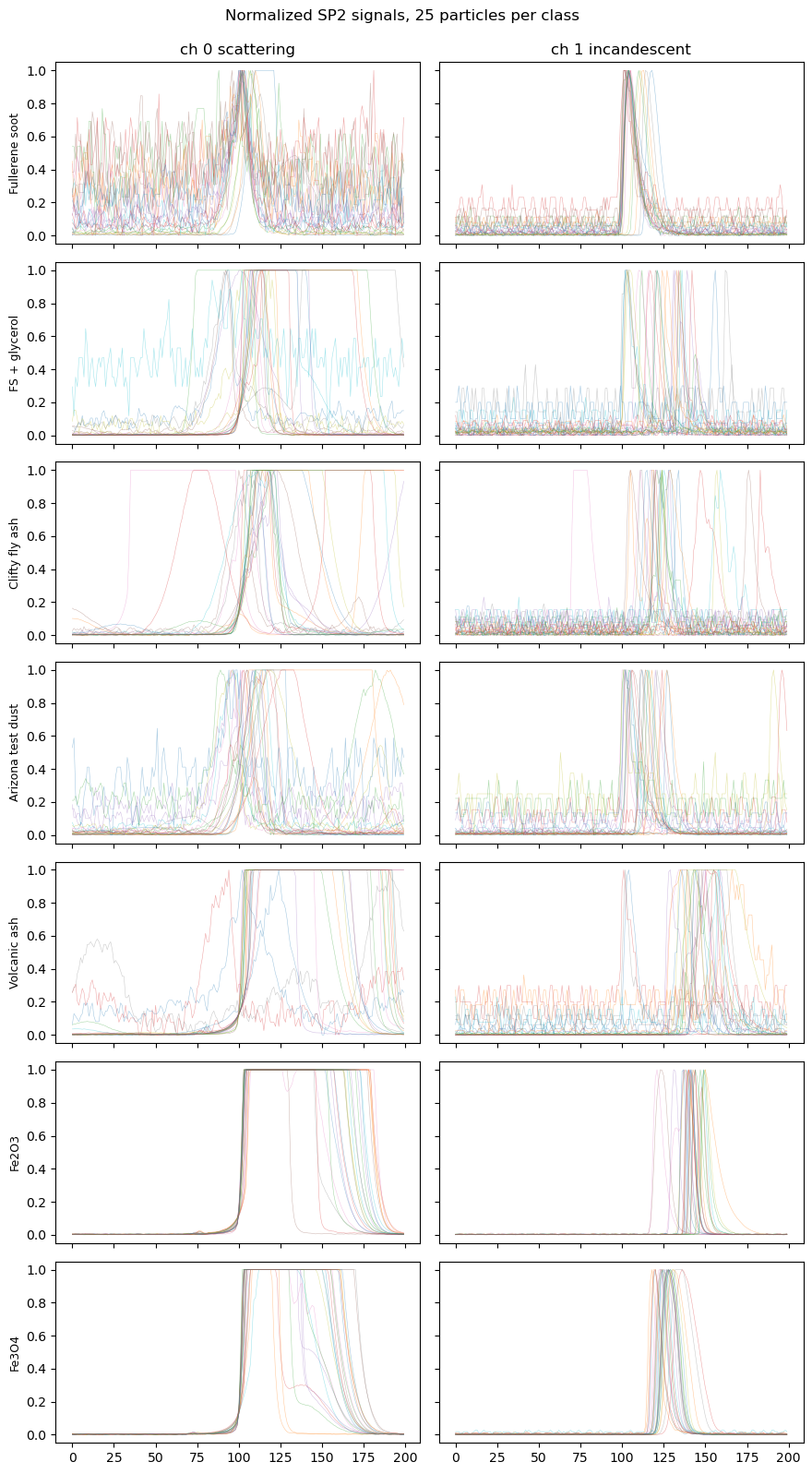
The shapes really do differ. Fullerene soot gives a narrow, symmetric incandescence peak and almost no scattering signal at all (its scattering trace is pure detector noise, which the normalization then stretches to fill the axis). The iron oxides give a broad, flat-topped scattering trace (the detector is saturated) and a later, wider incandescence peak. The dusts are messy and heterogeneous, because “Arizona test dust” is not one material but a mixture of mineral grains.

Those are exactly the features a human analyst would point at. Now let us see what the models find.

---

Example 1: a VAE latent space for seven aerosol types

A variational autoencoder squeezes each signal through a narrow bottleneck and reconstructs it from the other side. Nothing in the training objective mentions the aerosol type: the VAE never sees y. If the seven classes end up in different regions of the bottleneck, that is the model discovering differences between the different classes of aerosols on its own.

All three examples work on channel 1, the incandescent trace, which is the signal the SP2 records as a particle burns up. The paper trains a separate VAE on each channel; we keep to one so that the same 200-point input feeds all three models.

We use a 2-dimensional latent space, so we can simply plot it. (The paper found 3 dimensions optimal; you will see below that going from 2 to 3 buys a little accuracy and costs the ability to make this plot.)

The VAE encoder outputs a mean and a log-variance for each latent coordinate, and we sample from that Gaussian during training. The loss is the usual sum of a reconstruction term and a KL term that pulls the posterior towards a standard normal:

tf.random.set_seed(0)     # seed each example separately, so they stay independent
LATENT_DIM = 2


class Sampling(layers.Layer):
    "Draw z ~ N(mu, sigma^2) using the reparameterisation trick."
    def call(self, inputs):
        mu, logvar = inputs
        return mu + tf.exp(0.5 * logvar) * tf.random.normal(tf.shape(mu))


x_in = keras.Input((T, 1))
h = layers.Flatten()(x_in)
h = layers.Dense(256, activation="relu")(h)
h = layers.Dense(128, activation="relu")(h)
z_mean = layers.Dense(LATENT_DIM, name="z_mean")(h)
z_logvar = layers.Dense(LATENT_DIM, name="z_logvar")(h)
encoder = keras.Model(x_in, [z_mean, z_logvar, Sampling()([z_mean, z_logvar])],
                      name="encoder")

z_in = keras.Input((LATENT_DIM,))
g = layers.Dense(128, activation="relu")(z_in)
g = layers.Dense(256, activation="relu")(g)
g = layers.Dense(T, activation="sigmoid")(g)
decoder = keras.Model(z_in, layers.Reshape((T, 1))(g), name="decoder")

encoder.summary()

Model: "encoder"

__________________________________________________________________________________________________

 Layer (type)                Output Shape                 Param #   Connected to                  

==================================================================================================

 input_1 (InputLayer)        [(None, 200, 1)]             0         []                            

 flatten (Flatten)           (None, 200)                  0         ['input_1[0][0]']             

 dense (Dense)               (None, 256)                  51456     ['flatten[0][0]']             

 dense_1 (Dense)             (None, 128)                  32896     ['dense[0][0]']               

 z_mean (Dense)              (None, 2)                    258       ['dense_1[0][0]']             

 z_logvar (Dense)            (None, 2)                    258       ['dense_1[0][0]']             

 sampling (Sampling)         (None, 2)                    0         ['z_mean[0][0]',              

                                                                     'z_logvar[0][0]']            

==================================================================================================

Total params: 84868 (331.52 KB)

Trainable params: 84868 (331.52 KB)

Non-trainable params: 0 (0.00 Byte)

__________________________________________________________________________________________________

class VAE(keras.Model):
    def __init__(self, encoder, decoder):
        super().__init__()
        self.encoder, self.decoder = encoder, decoder
        self.tracker = keras.metrics.Mean(name="loss")

    def train_step(self, x):
        with tf.GradientTape() as tape:
            mu, logvar, z = self.encoder(x)
            reconstruction = self.decoder(z)
            rec_loss = tf.reduce_sum(tf.square(x - reconstruction), axis=[1, 2])
            kl_loss = -0.5 * tf.reduce_sum(
                1 + logvar - tf.square(mu) - tf.exp(logvar), axis=1)
            loss = tf.reduce_mean(rec_loss + kl_loss)
        self.optimizer.apply_gradients(
            zip(tape.gradient(loss, self.trainable_weights), self.trainable_weights))
        self.tracker.update_state(loss)
        return {"loss": self.tracker.result()}


vae = VAE(encoder, decoder)
vae.compile(optimizer=keras.optimizers.legacy.Adam(1e-3))

if not load_if_saved(vae_encoder=encoder, vae_decoder=decoder):
    t0 = time.time()
    history = vae.fit(X1, epochs=60, batch_size=128, verbose=0)
    print(f"trained in {time.time() - t0:.0f} s, "
          f"final loss {history.history['loss'][-1]:.2f}")
    save_weights(vae_encoder=encoder, vae_decoder=decoder)

loaded weights/vae_encoder.h5, weights/vae_decoder.h5 - delete these to train again

First a sanity check: can two numbers really rebuild a 200-point signal?

Z = encoder.predict(X1, verbose=0)[0]       # use the posterior mean as "the" code
recon = decoder.predict(Z, verbose=0)

fig, axes = plt.subplots(1, 5, figsize=(14, 2.6), sharex=True, sharey=True)
for ax, i in zip(axes, np.random.default_rng(3).choice(len(X1), 5, replace=False)):
    ax.plot(X1[i, :, 0], lw=1, label="real")
    ax.plot(recon[i, :, 0], lw=1, label="VAE reconstruction")
    ax.set_title(CLASSES[y[i]], fontsize=8)
axes[0].set_ylabel("ch 1 incandescent"); axes[0].legend(fontsize=7)
plt.tight_layout(); plt.show()

Two numbers get you a lot, but not everything. The peak lands in the right place almost every time, and for the narrow-peaked soots the reconstruction is close to exact. Two failure modes show up clearly. The reconstructed peak is often too short, most visibly for Fe2O3, where a saturated trace comes back at roughly half height. And anything unusual is dropped: a particle whose peak arrives unusually late, or which incandesces twice, gets reconstructed as a single peak in the ordinary place. That is a two-number bottleneck doing exactly what it should, spending its capacity on what is common across 8096 signals.

The reconstructions are also smooth: the high-frequency detector noise in the real traces is gone, because noise is by definition not compressible.

Now the plot we came for. Color each particle’s latent code by its true class:

fig, ax = plt.subplots(figsize=(7, 6))
for c in range(7):
    m = y == c
    ax.scatter(Z[m, 0], Z[m, 1], s=5, alpha=0.5, label=CLASSES[c])
ax.set_xlabel("$z_1$"); ax.set_ylabel("$z_2$")
ax.legend(markerscale=3, fontsize=8)
ax.set_title("VAE latent space, colored by aerosol type (labels never used in training)")
plt.tight_layout(); plt.show()

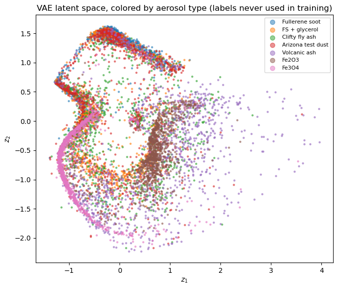
Structure, and more of it than the raw traces might lead you to expect. Three things are worth picking out.

The two soots pile into one tight cluster, at the far end of the \(z_1\) axis, with Arizona test dust mixed into the same knot. These are the narrow, symmetric, early-peaking signals, and the model puts them all in nearly the same place.

The two iron oxides each get their own filament, and the two filaments are distinct from each other: Fe3O4 traces one dense arc and Fe2O3 another, running in a different direction. This is the pair the paper singles out, so it is worth noting that an unsupervised model separates them on signal shape alone.

The dusts and volcanic ash spread out diffusely across the rest of the map rather than forming a cluster, which is what heterogeneous material should look like: “Arizona test dust” is not one substance but a mixture of mineral grains.

(A VAE’s latent axes have no fixed sign or ordering, so if you re-run the training your map may come out rotated or mirrored relative to this one. Only the relative arrangement is meaningful.)

To read the map, decode a grid of latent coordinates and see what signal each point of the plane corresponds to. This is the VAE equivalent of looking at principal component loadings:

from scipy.stats import norm

d = 9
gx = norm.ppf(np.linspace(0.05, 0.95, d))       # evenly spaced in probability
grid = np.array([[a, b] for b in gx[::-1] for a in gx], dtype="float32")
manifold = decoder.predict(grid, verbose=0)

fig, axes = plt.subplots(d, d, figsize=(9, 9), sharex=True, sharey=True)
for k, ax in enumerate(axes.ravel()):
    ax.plot(manifold[k, :, 0], lw=0.8, color="tab:red")
    ax.set_xticks([]); ax.set_yticks([])
fig.suptitle("Incandescent signals decoded from a grid over the latent space")
plt.tight_layout(); plt.show()

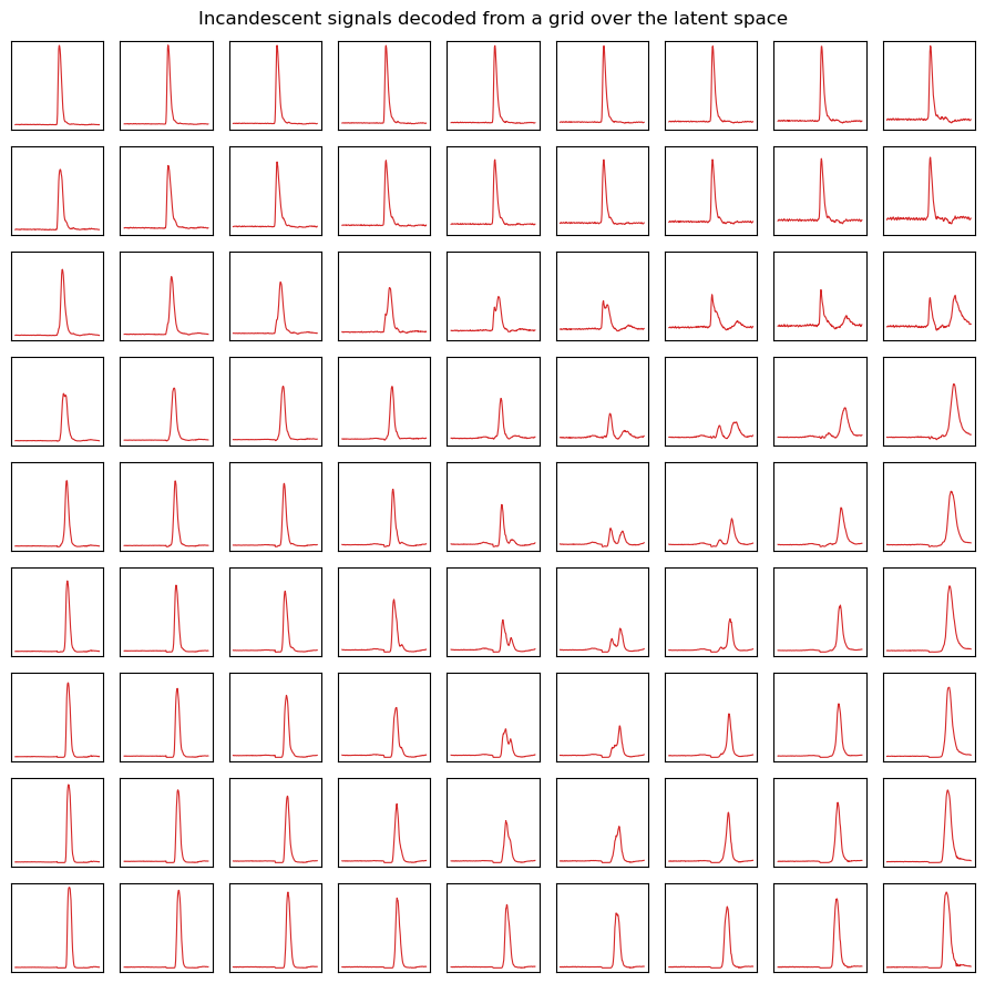
The manifold is smooth and physically interpretable, and this is the real payoff of a VAE over a plain autoencoder. Moving across the grid, the peak slides later in the time window. Moving down it, the trace sharpens and the baseline noise falls away. And there is a pocket in the upper middle where the decoder produces double-peaked signals, the shape a particle makes when it incandesces twice. Every point of the plane decodes to a plausible SP2 signal, not just the points where training data happened to land.

Finally, a number instead of an impression. If the latent space really organizes the classes, a simple nearest-neighbor classifier on the two latent coordinates should do far better than chance:

from sklearn.neighbors import KNeighborsClassifier
from sklearn.model_selection import cross_val_score

knn_latent = cross_val_score(KNeighborsClassifier(15), Z, y, cv=3).mean()
knn_raw = cross_val_score(KNeighborsClassifier(15), X1[:, :, 0], y, cv=3).mean()

print(f"15-NN accuracy on the {LATENT_DIM} latent coordinates : {knn_latent:.3f}")
print(f"15-NN accuracy on all {T} raw numbers            : {knn_raw:.3f}")
print(f"chance                                       : {1/7:.3f}")

15-NN accuracy on the 2 latent coordinates : 0.512
15-NN accuracy on all 200 raw numbers            : 0.578
chance                                       : 0.143

Two coordinates retain most of what the full 200-point trace carries, at a 100-fold compression. Neither number is close to 1.0, and it is worth being clear about why.

Part of it is the science: several of these aerosols genuinely produce overlapping SP2 signatures once you take the peak height away, and quantifying that overlap is part of the paper’s contribution. But part of it is simply that we have handicapped the models, deliberately, to keep this tutorial runnable in a class session. We train on 8,096 signals out of the 42,960 incandescing particles in the test split alone, and the full data set also has train and validation splits we never download. And we use one of the instrument’s four channels, throwing away the scattering trace, the red incandescent channel, and the position-sensitive detector, along with the peak heights we normalized out. None of these models is being shown anything close to the information the SP2 actually records. Expect every number on this page to improve if you give them more.

Try it: set LATENT_DIM = 3 and re-run the three cells above. The classifier improves (the paper found 3 dimensions optimal) but you lose the plot. How much accuracy is a picture worth?

---

Example 2: a GAN as an anomaly detector for fullerene soot

Fullerene soot is the standard laboratory proxy for atmospheric black carbon, and it is what an SP2 is normally calibrated against. Suppose we deploy an instrument in the field: we would like it to tell us when a particle is not behaving like the soot we calibrated on: perhaps it is dust, or an iron oxide, or something we have never characterized.

That is a one-class problem. We cannot train a classifier for “everything that isn’t soot”, because we do not have examples of everything. But we can learn what soot looks like and measure how badly a new signal fits.

A GAN gives us exactly that. Train the generator on fullerene soot alone and it learns to produce soot signals and nothing else. Then for a new signal, search the latent space for the code whose generated signal comes closest. If even the best match is poor, the signal is anomalous. This is the AnoGAN recipe (Schlegl et al. 2017), originally developed for finding disease markers in retinal scans.

tf.random.set_seed(0)
NOISE_DIM = 16
Xg = X1                                 # the same incandescent signals as the VAE

rng2 = np.random.default_rng(1)
soot = np.flatnonzero(y == 0)
rng2.shuffle(soot)

gan_train = Xg[soot[:1000]]             # the GAN sees ONLY fullerene soot
test_idx = np.concatenate([soot[1000:1200]] +
    [rng2.choice(np.flatnonzero(y == c), 200, replace=False) for c in range(1, 7)])
X_test, y_test = Xg[test_idx], y[test_idx]

print("GAN training set (fullerene soot only):", gan_train.shape)
print("held-out test set (200 per class)     :", X_test.shape)

GAN training set (fullerene soot only): (1000, 200, 1)
held-out test set (200 per class)     : (1400, 200, 1)

generator = keras.Sequential([
    keras.Input((NOISE_DIM,)),
    layers.Dense(25 * 64), layers.LeakyReLU(0.2), layers.Reshape((25, 64)),
    layers.Conv1DTranspose(64, 5, strides=2, padding="same"), layers.LeakyReLU(0.2),
    layers.Conv1DTranspose(32, 5, strides=2, padding="same"), layers.LeakyReLU(0.2),
    layers.Conv1DTranspose(32, 5, strides=2, padding="same"), layers.LeakyReLU(0.2),
    layers.Conv1D(1, 5, padding="same", activation="sigmoid"),
], name="generator")

discriminator = keras.Sequential([
    keras.Input((T, 1)),
    layers.Conv1D(32, 5, strides=2, padding="same"), layers.LeakyReLU(0.2), layers.Dropout(0.3),
    layers.Conv1D(64, 5, strides=2, padding="same"), layers.LeakyReLU(0.2), layers.Dropout(0.3),
    layers.Conv1D(64, 5, strides=2, padding="same"), layers.LeakyReLU(0.2),
    layers.Flatten(), layers.Dense(1),
], name="discriminator")

generator.summary()

Model: "generator"

_________________________________________________________________

 Layer (type)                Output Shape              Param #   

=================================================================

 dense_5 (Dense)             (None, 1600)              27200     

 leaky_re_lu (LeakyReLU)     (None, 1600)              0         

 reshape_1 (Reshape)         (None, 25, 64)            0         

 conv1d_transpose (Conv1DTr  (None, 50, 64)            20544     

 anspose)                                                        

 leaky_re_lu_1 (LeakyReLU)   (None, 50, 64)            0         

 conv1d_transpose_1 (Conv1D  (None, 100, 32)           10272     

 Transpose)                                                      

 leaky_re_lu_2 (LeakyReLU)   (None, 100, 32)           0         

 conv1d_transpose_2 (Conv1D  (None, 200, 32)           5152      

 Transpose)                                                      

 leaky_re_lu_3 (LeakyReLU)   (None, 200, 32)           0         

 conv1d (Conv1D)             (None, 200, 1)            161       

=================================================================

Total params: 63329 (247.38 KB)

Trainable params: 63329 (247.38 KB)

Non-trainable params: 0 (0.00 Byte)

_________________________________________________________________

The training loop is the two-player game from the notes, written out explicitly because Keras has no built-in “fit a GAN”: one gradient step for the discriminator (real → 1, fake → 0), then one for the generator (fool the discriminator into saying 1).

bce = keras.losses.BinaryCrossentropy(from_logits=True)
opt_g = keras.optimizers.legacy.Adam(2e-4, beta_1=0.5)
opt_d = keras.optimizers.legacy.Adam(2e-4, beta_1=0.5)


@tf.function
def gan_step(real):
    n = tf.shape(real)[0]

    with tf.GradientTape() as tape:                       # discriminator
        fake = generator(tf.random.normal((n, NOISE_DIM)), training=True)
        d_loss = (bce(tf.ones((n, 1)), discriminator(real, training=True))
                  + bce(tf.zeros((n, 1)), discriminator(fake, training=True)))
    opt_d.apply_gradients(zip(tape.gradient(d_loss, discriminator.trainable_weights),
                              discriminator.trainable_weights))

    with tf.GradientTape() as tape:                       # generator
        fake = generator(tf.random.normal((n, NOISE_DIM)), training=True)
        g_loss = bce(tf.ones((n, 1)), discriminator(fake, training=True))
    opt_g.apply_gradients(zip(tape.gradient(g_loss, generator.trainable_weights),
                              generator.trainable_weights))
    return d_loss, g_loss


if not load_if_saved(gan_generator=generator, gan_discriminator=discriminator):
    t0 = time.time()
    ds = tf.data.Dataset.from_tensor_slices(gan_train).shuffle(1000).batch(64)
    history = []
    for epoch in range(60):
        epoch_losses = []
        for batch in ds:
            d_loss, g_loss = gan_step(batch)
            epoch_losses.append([float(d_loss), float(g_loss)])
        history.append(np.mean(epoch_losses, axis=0))       # mean over the epoch
        if epoch % 20 == 0:
            print(f"  epoch {epoch:3d}  d_loss {history[-1][0]:.3f}  "
                  f"g_loss {history[-1][1]:.3f}")
    print(f"trained in {time.time() - t0:.0f} s")
    save_weights(gan_generator=generator, gan_discriminator=discriminator)
    np.save(f"{WEIGHTS}/gan_history.npy", np.array(history))

gan_history = np.load(f"{WEIGHTS}/gan_history.npy")

  epoch   0  d_loss 1.296  g_loss 0.814

  epoch  20  d_loss 1.264  g_loss 0.803

  epoch  40  d_loss 1.352  g_loss 0.716

trained in 25 s
saved weights/gan_generator.h5, weights/gan_discriminator.h5

fig, ax = plt.subplots(figsize=(7, 3.2))
ax.plot(gan_history[:, 0], label="discriminator")
ax.plot(gan_history[:, 1], label="generator")
ax.set_xlabel("epoch"); ax.set_ylabel("loss (mean over the epoch)")
ax.set_title("The two players over 60 epochs")
ax.legend()
plt.tight_layout(); plt.show()

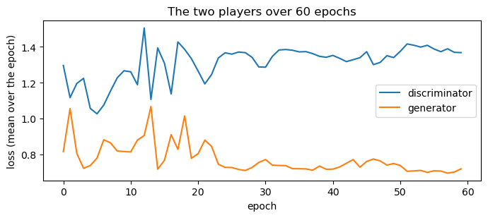
Read that plot the way you would not read a supervised loss curve. Neither line falls towards zero. Both bounce around for the first twenty epochs or so, then settle onto roughly flat plateaus, the discriminator near 1.35 and the generator near 0.72, and stay there. That is what success looks like here: the two networks are chasing each other, and a GAN that is training well looks like a stalemate. A discriminator loss collapsing towards zero would mean the generator had stopped fooling it. Since the loss cannot tell you whether the samples are any good, judge it by the samples.

fig, axes = plt.subplots(1, 2, figsize=(11, 3), sharey=True)
for i in range(6):
    axes[0].plot(gan_train[rng2.integers(len(gan_train)), :, 0], lw=1)
    axes[1].plot(generator(tf.random.normal((1, NOISE_DIM)))[0, :, 0], lw=1)
axes[0].set_title("real fullerene soot")
axes[1].set_title("GAN samples")
plt.tight_layout(); plt.show()

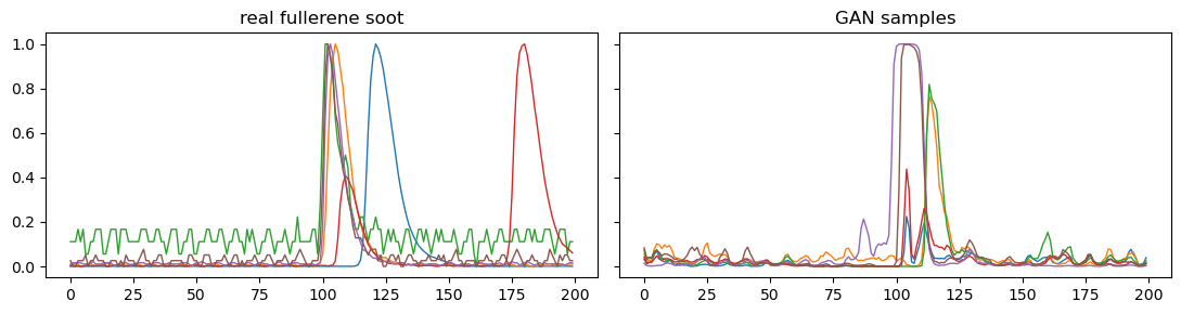
The generator has learned the narrow peak, its typical position, and even the level of the detector noise floor around it.

Scoring a new signal

The generator maps a latent code to a signal, but there is no inverse. AnoGAN’s answer is to search: hold the generator fixed and run gradient descent on the latent code \(z\) until \(G(z)\) matches the query signal as well as it can. The final mismatch is the anomaly score. We use the standard combination of a direct residual and a “feature” residual measured in the discriminator’s last hidden layer, which compares signals the way the discriminator learned to.

All 1400 test signals are optimised at once as one batch, so this takes seconds rather than minutes.

features = keras.Model(discriminator.input, discriminator.layers[-2].output)


def anomaly_score(x, steps=200, lr=0.05):
    "Search for the latent code whose generated signal best matches x."
    x = tf.constant(x, tf.float32)
    z = tf.Variable(tf.random.normal((x.shape[0], NOISE_DIM)))
    opt = keras.optimizers.legacy.Adam(lr)
    fx = features(x)
    for _ in range(steps):
        with tf.GradientTape() as tape:
            fake = generator(z)
            score = (tf.reduce_mean(tf.abs(x - fake), axis=[1, 2])
                     + 0.1 * tf.reduce_mean(tf.abs(fx - features(fake)), axis=1))
            total = tf.reduce_sum(score)
        opt.apply_gradients([(tape.gradient(total, z), z)])
    return score.numpy(), generator(z).numpy()


t0 = time.time()
score, best_fit = anomaly_score(X_test)
print(f"scored {len(X_test)} signals in {time.time() - t0:.0f} s")

scored 1400 signals in 36 s

from sklearn.metrics import roc_auc_score, roc_curve

is_anomaly = (y_test != 0).astype(int)
auc = roc_auc_score(is_anomaly, score)
print(f"AUC, fullerene soot vs everything else: {auc:.3f}\n")
for c in np.argsort([np.median(score[y_test == c]) for c in range(7)]):
    print(f"  {CLASSES[c]:20s} median score {np.median(score[y_test == c]):.4f}")

AUC, fullerene soot vs everything else: 0.793

  Fullerene soot       median score 0.0210
  Arizona test dust    median score 0.0322
  Fe2O3                median score 0.0345
  FS + glycerol        median score 0.0372
  Clifty fly ash       median score 0.0487
  Fe3O4                median score 0.0520
  Volcanic ash         median score 0.0576

fig, axes = plt.subplots(1, 2, figsize=(12, 4))
for c in range(7):
    axes[0].hist(score[y_test == c], bins=25, histtype="step", lw=1.5, label=CLASSES[c])
axes[0].set_xlabel("anomaly score"); axes[0].set_ylabel("count")
axes[0].legend(fontsize=7); axes[0].set_title("anomaly score by class")

fpr, tpr, _ = roc_curve(is_anomaly, score)
axes[1].plot(fpr, tpr); axes[1].plot([0, 1], [0, 1], "k--", lw=0.8)
axes[1].set_xlabel("false positive rate"); axes[1].set_ylabel("true positive rate")
axes[1].set_title(f"flagging non-soot particles: AUC = {auc:.3f}")
plt.tight_layout(); plt.show()

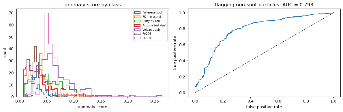
Fullerene soot has the lowest median score of the seven, which is what a one-class detector is supposed to deliver, but look at the overlap. Plenty of Arizona test dust and glycerol-coated soot particles score as low as real soot does. That overlap is the difference between an AUC near 0.8 and an AUC near 1.0, and it is a genuine property of the data rather than a shortcoming of the training run: some of these particles produce incandescence traces that are essentially indistinguishable from soot once the peak height is normalized away.

Note also that the ranking of the six anomalous classes carries no physical meaning. The score measures distance from soot in signal space, and a class does not have to be chemically far from soot to land far away there.

Looking at what the generator actually produced for each query makes the failure mode concrete:

picks = [(0, 0), (0, 1), (1, 0), (2, 0), (3, 0), (4, 0), (5, 0), (6, 0)]
fig, axes = plt.subplots(2, 4, figsize=(13, 4.5), sharex=True, sharey=True)
for ax, (c, k) in zip(axes.ravel(), picks):
    i = np.flatnonzero(y_test == c)[k]
    ax.plot(X_test[i, :, 0], lw=1, label="real")
    ax.plot(best_fit[i, :, 0], lw=1, label="closest GAN sample")
    ax.set_title(f"{CLASSES[y_test[i]]}  score {score[i]:.3f}", fontsize=8)
axes[0, 0].legend(fontsize=7)
fig.suptitle("What a soot-only generator can and cannot reproduce")
plt.tight_layout(); plt.show()

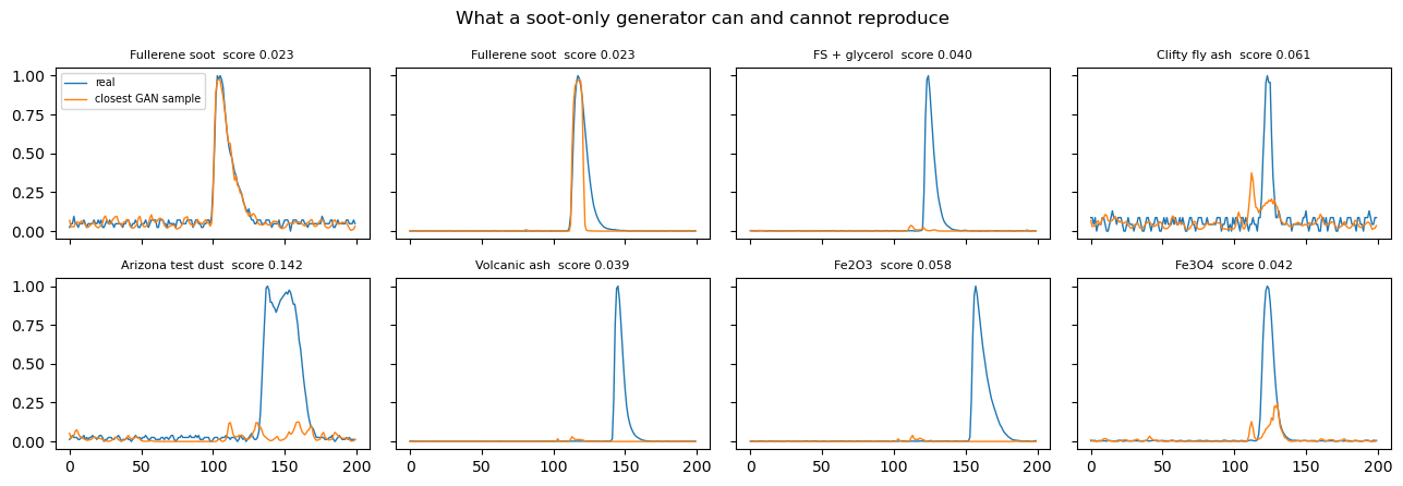
For fullerene soot the generator finds a near-perfect match, noise floor and all. For the other classes it cannot: the peak is in the wrong place, or too wide, and in the worst cases the search gives up and returns something nearly flat. That residual is the anomaly score.

Try it: train the same GAN on Fe2O3 instead (y == 5) and score the rest. Which classes now look normal? Does fullerene soot become the anomaly?

---

Example 3: a conditional diffusion model for all seven classes

The VAE and the GAN both learned one distribution. A conditional generative model learns a family of distributions indexed by a label.

“Conditional” in machine learning means the model takes an extra input alongside its usual one and its output depends on that input. Here the extra input is the aerosol class, so instead of learning “what does an SP2 signal look like?” the model learns “what does an SP2 signal of class c look like?” The label is not something the model predicts, the way a classifier would; it is something we hand it, and it steers what comes out. That is what lets us ask for “an Fe2O3 signal” or “a fullerene soot signal” on demand. That is what makes generative models useful for augmenting training sets, for simulating instruments, and for testing analysis pipelines against synthetic data with known ground truth.

We build a denoising diffusion model on the incandescent channel. The recipe:

• Forward process: add Gaussian noise to a real signal in \(T = 200\) small steps until nothing is left but noise. This needs no training, since it is a fixed schedule.

• Reverse process: train a network to predict, given a noisy signal, the time step, and the class label, what noise was added. Generation starts from pure noise and subtracts the predicted noise 200 times.

Diffusion models are far more stable to train than GANs, because the loss is an ordinary mean-squared error with no adversarial game. That is the main reason they took over image generation.

NUM_STEPS = 200
NULL_LABEL = 7                       # an eighth "no class specified" token, used below

betas = np.linspace(1e-4, 0.02, NUM_STEPS).astype("float32")   # noise added per step
alpha_bar = np.cumprod(1 - betas).astype("float32")            # signal surviving to step t
alpha_bar_tf = tf.constant(alpha_bar)

X_diff = (2 * X1 - 1).astype("float32")                        # rescale to [-1, 1]

fig, axes = plt.subplots(1, 4, figsize=(13, 2.6), sharey=True)
i = np.flatnonzero(y == 0)[0]
for ax, t in zip(axes, [0, 40, 100, 199]):
    noisy = (np.sqrt(alpha_bar[t]) * X_diff[i, :, 0]
             + np.sqrt(1 - alpha_bar[t]) * np.random.randn(T))
    ax.plot(noisy, lw=0.8); ax.set_title(f"t = {t}", fontsize=9)
fig.suptitle("Forward process: a fullerene soot signal dissolving into noise")
plt.tight_layout(); plt.show()

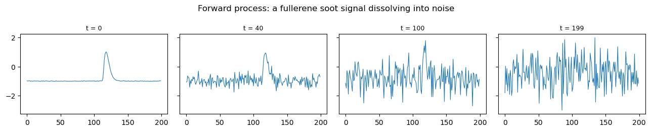
The denoiser is a small 1-D U-Net: three resolutions down, two back up, with skip connections. Two extra inputs are mixed into every block as a learned embedding: the time step (encoded with sinusoids, as in a transformer) and the class label. A constant position ramp is concatenated to the input as well; without it the convolutions are nearly translation-invariant and the model puts the peak in the wrong place.

def build_denoiser():
    x_in = keras.Input((T, 1))
    t_in = keras.Input((), dtype="int32")
    y_in = keras.Input((), dtype="int32")

    freqs = tf.exp(tf.linspace(0.0, -4.0, 32) * tf.math.log(10.0))
    ang = tf.cast(t_in, tf.float32)[:, None] * freqs[None, :]
    emb = layers.Dense(64, activation="swish")(tf.concat([tf.sin(ang), tf.cos(ang)], -1))
    emb = emb + layers.Embedding(8, 64)(y_in)          # 7 classes + the null token
    emb = layers.Dense(64, activation="swish")(emb)

    def block(h, ch):
        h = layers.Conv1D(ch, 5, padding="same", activation="swish")(h)
        h = h + layers.Dense(ch)(emb)[:, None, :]      # inject time + class
        return layers.Conv1D(ch, 5, padding="same", activation="swish")(h)

    pos = tf.linspace(-1.0, 1.0, T)[None, :, None] * tf.ones_like(x_in[:, :, :1])
    h1 = block(layers.Concatenate()([x_in, pos]), 32)          # 200 points
    h2 = block(layers.AveragePooling1D(2)(h1), 64)             # 100
    h3 = block(layers.AveragePooling1D(2)(h2), 128)            #  50
    u2 = block(layers.Concatenate()([layers.UpSampling1D(2)(h3), h2]), 64)
    u1 = block(layers.Concatenate()([layers.UpSampling1D(2)(u2), h1]), 32)
    return keras.Model([x_in, t_in, y_in], layers.Conv1D(1, 5, padding="same")(u1))


tf.random.set_seed(0)
denoiser = build_denoiser()
print("denoiser parameters:", denoiser.count_params())

denoiser parameters: 291873

One trick in the training step: 10 % of the time we replace the real label with the null token, so the same network learns both the class-conditional and the unconditional denoiser. That is what makes classifier-free guidance possible at sampling time, and we will measure below how much it matters.

EPOCHS = 80
steps_total = EPOCHS * int(np.ceil(len(X_diff) / 128))
opt_dn = keras.optimizers.legacy.Adam(
    keras.optimizers.schedules.CosineDecay(1e-3, steps_total, alpha=0.05))


@tf.function
def diffusion_step(x0, label):
    n = tf.shape(x0)[0]
    label = tf.where(tf.random.uniform((n,)) < 0.1, NULL_LABEL, label)   # label dropout
    t = tf.random.uniform((n,), 0, NUM_STEPS, dtype=tf.int32)
    a = tf.gather(alpha_bar_tf, t)[:, None, None]
    eps = tf.random.normal(tf.shape(x0))
    x_t = tf.sqrt(a) * x0 + tf.sqrt(1 - a) * eps          # jump straight to step t
    with tf.GradientTape() as tape:
        loss = tf.reduce_mean(tf.square(eps - denoiser([x_t, t, label], training=True)))
    opt_dn.apply_gradients(zip(tape.gradient(loss, denoiser.trainable_weights),
                               denoiser.trainable_weights))
    return loss


if not load_if_saved(diffusion_denoiser=denoiser):
    t0 = time.time()
    ds = tf.data.Dataset.from_tensor_slices(
        (X_diff, y.astype("int32"))).shuffle(8000).batch(128)
    running = None
    for epoch in range(EPOCHS):
        for xb, yb in ds:
            l = float(diffusion_step(xb, yb))
            running = l if running is None else 0.99 * running + 0.01 * l
        if epoch % 10 == 0:
            print(f"  epoch {epoch:3d}  loss {running:.4f}  ({time.time() - t0:.0f} s)")
    print(f"trained in {time.time() - t0:.0f} s")
    save_weights(diffusion_denoiser=denoiser)

loaded weights/diffusion_denoiser.h5 - delete these to train again

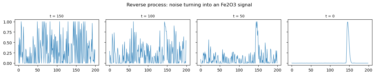
Sampling

Start from pure noise and walk the schedule backwards. With classifier-free guidance we run the denoiser twice at each step, once with the class label and once with the null token, and extrapolate away from the unconditional prediction:

\[\hat\epsilon = (1 + w)\,\epsilon_\theta(x_t, t, c) - w\,\epsilon_\theta(x_t, t, \varnothing)\]

The guidance weight \(w\) trades diversity for class fidelity. \(w = 0\) is ordinary conditional sampling. We generate 20 signals per class at three guidance weights so we can compare them later; the figures below use \(w = 3\).

def sample(labels, guidance=3.0, snapshots=()):
    n = len(labels)
    labels = tf.constant(np.asarray(labels, "int32"))
    null = tf.fill((n,), NULL_LABEL)
    x = tf.random.normal((n, T, 1))
    saved = {}
    for i in range(NUM_STEPS - 1, -1, -1):
        t_i = tf.fill((n,), i)
        eps = denoiser([x, t_i, labels], training=False)
        if guidance:
            eps = ((1 + guidance) * eps
                   - guidance * denoiser([x, t_i, null], training=False))
        x = (x - betas[i] / np.sqrt(1 - alpha_bar[i]) * eps) / np.sqrt(1 - betas[i])
        if i > 0:
            x = x + np.sqrt(betas[i]) * tf.random.normal(tf.shape(x))
        if i in snapshots:
            saved[i] = np.clip((x.numpy() + 1) / 2, 0, 1)
    return np.clip((x.numpy() + 1) / 2, 0, 1), saved


labels = np.repeat(np.arange(7), 20)      # 20 signals of each class

t0 = time.time()
samples = {}
for w in [0.0, 1.0, 3.0]:
    samples[w], snaps = sample(labels, guidance=w, snapshots=(150, 100, 50))
fake = samples[3.0]
print(f"generated {len(labels)} signals at each of 3 guidance weights "
      f"in {time.time() - t0:.0f} s")

generated 140 signals at each of 3 guidance weights in 73 s

fig, axes = plt.subplots(1, 4, figsize=(13, 2.6), sharey=True)
i = np.flatnonzero(labels == 5)[0]
for ax, t in zip(axes, [150, 100, 50]):
    ax.plot(snaps[t][i, :, 0], lw=0.8); ax.set_title(f"t = {t}", fontsize=9)
axes[3].plot(fake[i, :, 0], lw=0.8); axes[3].set_title("t = 0", fontsize=9)
fig.suptitle("Reverse process: noise turning into an Fe2O3 signal")
plt.tight_layout(); plt.show()

fig, axes = plt.subplots(7, 2, figsize=(9, 16), sharex=True, sharey=True)
for c in range(7):
    for i in np.flatnonzero(y == c)[:6]:
        axes[c, 0].plot(X1[i, :, 0], lw=0.8)
    for i in np.flatnonzero(labels == c)[:6]:
        axes[c, 1].plot(fake[i, :, 0], lw=0.8)
    axes[c, 0].set_ylabel(CLASSES[c], fontsize=9)
axes[0, 0].set_title("real"); axes[0, 1].set_title("generated")
fig.suptitle("Incandescent channel, real vs. diffusion samples", y=0.995)
plt.tight_layout(); plt.show()

Did it actually condition on the class?

“Looks plausible” is not a result. Two checks.

First, a reference classifier: fit a nearest-neighbor classifier on the real incandescent signals, then ask it to label the generated ones. Its own cross-validated accuracy on real data is the natural yardstick.

reference = KNeighborsClassifier(15).fit(X1[:, :, 0], y)
ceiling = cross_val_score(KNeighborsClassifier(15), X1[:, :, 0], y, cv=3).mean()

pred = reference.predict(fake[:, :, 0])
print(f"reference classifier on real signals : {ceiling:.3f}  (chance {1/7:.3f})")
print(f"generated signals given their target : {(pred == labels).mean():.3f}\n")
for c in range(7):
    m = labels == c
    print(f"  asked for {CLASSES[c]:20s} got it {(pred[m] == c).mean():.2f} of the time;"
          f"  most common label: {CLASSES[np.bincount(pred[m], minlength=7).argmax()]}")

reference classifier on real signals : 0.578  (chance 0.143)
generated signals given their target : 0.593

  asked for Fullerene soot       got it 0.75 of the time;  most common label: Fullerene soot
  asked for FS + glycerol        got it 0.35 of the time;  most common label: Fullerene soot
  asked for Clifty fly ash       got it 0.75 of the time;  most common label: Clifty fly ash
  asked for Arizona test dust    got it 0.30 of the time;  most common label: Clifty fly ash
  asked for Volcanic ash         got it 0.70 of the time;  most common label: Volcanic ash
  asked for Fe2O3                got it 0.85 of the time;  most common label: Fe2O3
  asked for Fe3O4                got it 0.45 of the time;  most common label: Fe3O4

The classifier assigns the generated signals to the class they were asked for about as often as it gets real signals right. The conditioning is doing real work, and this is the number the extra training epochs bought: at half the training length it sat nearer 0.40.

Resist reading that as “the generated signals are indistinguishable from real ones”. It is partly a side effect of the guidance, which pushes samples towards the most typical example of each class, and a prototype is easier to classify than a real particle. What the number does establish is that the label input is genuinely controlling what comes out.

Second, compare summary statistics of the signal shape, the features a conventional SP2 analysis would extract, class by class:

real_pos, gen_pos = [], []
print(f"{'':22s}{'peak position':>18s}{'peak width':>16s}")
print(f"{'':22s}{'real':>9s}{'gen':>9s}{'real':>8s}{'gen':>8s}")
for c in range(7):
    r, g = X1[y == c, :, 0], fake[labels == c, :, 0]
    real_pos.append(np.median(r.argmax(1)))
    gen_pos.append(np.median(g.argmax(1)))
    print(f"  {CLASSES[c]:20s}{real_pos[-1]:9.0f}{gen_pos[-1]:9.0f}"
          f"{np.median((r > 0.5).sum(1)):8.0f}{np.median((g > 0.5).sum(1)):8.0f}")
print(f"\ncorrelation of the 7 median peak positions: "
      f"{np.corrcoef(real_pos, gen_pos)[0, 1]:.2f}")

                           peak position      peak width
                           real      gen    real     gen
  Fullerene soot            104      102       8      10
  FS + glycerol             119      106       7       8
  Clifty fly ash            125      141       7      26
  Arizona test dust         112      105       7       8
  Volcanic ash              138      138      10      36
  Fe2O3                     142      150       6       6
  Fe3O4                     125      128       9      14

correlation of the 7 median peak positions: 0.90

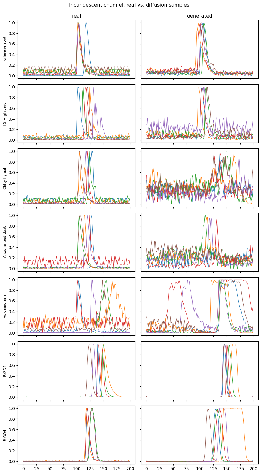
The generated peak positions track the real ones across classes: the model has learned, from the label alone, that an Fe2O3 particle incandesces later in the laser beam than a fullerene soot particle does.

The peak widths are less faithful: the generated peaks come out wider than the real ones for every class. That is the usual signature of a diffusion model trained for a few minutes rather than a few hours. It learns where the peak goes before it learns how sharp it is.

Read the per-class table with care, for two reasons. Twenty signals per class is a small sample, so those numbers move around between runs. And there is a systematic quirk: the classes that barely incandesce (Clifty fly ash, Arizona test dust) have genuinely noise-dominated real traces, so any generated signal that comes out noisy tends to get labelled as one of them, whether or not that is what we asked for. Look at the figure and the table together: the figure is where you can see that the model reproduces Fe2O3 and Fe3O4 cleanly and the weakly-incandescing classes poorly.

Finally, the guidance ablation, on the three sets of samples we generated above:

for w, f in samples.items():
    acc = (reference.predict(f[:, :, 0]) == labels).mean()
    print(f"guidance w = {w}:  class accuracy {acc:.3f}")

guidance w = 0.0:  class accuracy 0.357
guidance w = 1.0:  class accuracy 0.386
guidance w = 3.0:  class accuracy 0.593

Guidance buys real class fidelity, and it costs only a second network evaluation per sampling step. It is not free in general, since pushed far enough it collapses the diversity of the samples, so that every “Fe2O3” starts to look like the same Fe2O3, but at these settings the trade is clearly worth making.

Treat these numbers as a trend rather than as precise measurements: each is based on 140 generated signals, so there is several percent of scatter between runs. The gap between no guidance and \(w = 3\) survives that scatter; the intermediate point does not always sit neatly between the two.

One caveat worth stating plainly, because it is easy to hide. This is a small model trained for a few minutes, and how well it works varies between training runs. Across seven runs we measured the peak-position correlation between 0.82 and 0.99 most of the time, but one run came out near zero: the conditioning simply failed to take, while the training loss looked completely normal. The loss will not warn you, so the correlation printed above is the check. If yours comes out low, delete weights/diffusion_denoiser.h5 and train again. (Halving the learning rate makes this worse, not better; doubling the epochs from 40 to 80 is what bought the class accuracy you see here.)

Try it: push the guidance to w = 10 and look at the samples. Can you see the diversity collapse in the figure before you see it in the number?

---

Wrapping up

Three architectures, one instrument, three different jobs:

model	what it learned	what we used it for
VAE	a smooth 2-D coordinate system for signal shape	visualizing and quantifying how separable the seven aerosols are
GAN	the distribution of fullerene soot alone	flagging particles that do not behave like the calibration material
conditional diffusion	one distribution per class	generating labelled synthetic signals on demand

Some things worth carrying away:

• None of the three ever saw a label during training, except the diffusion model, and it used the label only as a conditioning input, never as a target to predict. These are generative, not discriminative, models.

• Preprocessing decided most of the outcome. Normalizing away the peak height was a deliberate choice to isolate signal shape; it also threw away the single most discriminating feature in the data set. Every number above would be higher if we had kept it.

• These models are underfed, on purpose. They see 8,096 signals and one of four instrument channels, because the whole tutorial has to run in a class session on a laptop. That, as much as anything intrinsic to the aerosols, is why none of the scores is spectacular. Treat the numbers here as a floor, not as what the method can do.

• Verify generative models with numbers, not with pictures. Plausible-looking samples are easy; samples that a classifier trained on real data agrees with are not.

Exercises

1. Add channel 2 (the red incandescent detector) to the VAE input and compute the color ratio (peak ch1 divided by peak ch2), which is the classical SP2 proxy for particle temperature. Is the color ratio recoverable from the latent coordinates?

2. The two iron oxides, Fe2O3 and Fe3O4, are the pair the paper found most interesting. Train a VAE on those two classes alone with a 2-D latent space. Do they separate?

3. Use the trained diffusion model as a data-augmentation engine: generate 500 signals per class, train a supervised classifier on the synthetic data only, and test it on real data. How close does it get to a classifier trained on real data?

4. The GAN in Example 2 was trained on 1000 signals. Retrain it on 100 and on 5000 and plot the anomaly-detection AUC against training-set size.

5. Lamb (2019) classified these same aerosols with a random forest on hand-built features (peak height, color ratio, peak width). Train one on the scalar features you can compute from X and peak, and compare its accuracy with the 0.58 the VAE latent space gave us. Where does the supervised model win, and what does it need that the VAE did not?

Note that all three trained models are cached in weights/. Delete a file there to retrain that model from scratch; leave them alone and the notebook re-runs in under a minute.

References

• Lamb, K. D. (2019), Classification of iron oxide aerosols by a single particle soot photometer using supervised machine learning, Atmospheric Measurement Techniques 12, 3885–3906, https://amt.copernicus.org/articles/12/3885/2019/. The paper that introduced this laboratory data set, and classified it with a random forest.

• Doshi, A. and Lamb, K. D. (2025), Unsupervised classification of absorbing aerosols with the SP2 via a variational autoencoder, Atmospheric Measurement Techniques 18, 7767, https://amt.copernicus.org/articles/18/7767/2025/amt-18-7767-2025.html. Code: kdlamb/SP2-VAE. Data: https://zenodo.org/records/15800436.