Generative Models and Uncertainty

The deep learning architectures we have seen so far, the artificial neural network, the convolutional neural network, and the recurrent neural network, are all discriminative: given an input, they predict a single output. This page begins the Advanced Topics unit with generative modeling, where a model instead predicts a distribution of possible outputs. We will:

• Define generative modeling and contrast it with what we have seen before.

• Distinguish aleatoric from epistemic uncertainty.

• Survey the main ways of adding uncertainty to machine learning models.

• Learn to evaluate uncertainty estimates, with the spread vs. skill plot and the continuous ranked probability score (CRPS).

The next page covers two state-of-the-art generative architectures, GANs and diffusion models, and the page after that covers a third, the variational autoencoder, together with the scientific uses of its latent representations.

Why include uncertainty?

Consider a downscaling problem from the satellite literature (Leinonen et al. 2020). We observe a low resolution satellite image of rain rates: each coarse pixel averages over many fine ones, so information about the small scale structure has been lost. Now we ask a machine learning model to reconstruct the high resolution rain field. There is no longer a single right answer: many different fine scale fields would average to exactly the same coarse image, and the low resolution input does not contain enough information to discriminate between them.

A model trained to output one answer must collapse all of those possibilities onto a single field. Without including uncertainty, machine learning models can be overconfident in their predictions: the one field they return may look plausible while being far from the truth, and nothing in the output warns us. What we would rather have is the distribution of rain fields consistent with the input. An ensemble of samples from that distribution tells us what the probable rain rates are, and how much they could vary.

That is what a generative model is: a statistical model that predicts a joint probability distribution over its variables, so that given an input \(x\) it can return a conditional distribution \(p(y \mid x)\) of outputs rather than a single output vector \(y\).

Two kinds of uncertainty

Machine learning distinguishes two sources of uncertainty (Abdar et al. 2021):

• Aleatoric uncertainty is the irreducible scatter in the system itself, for example measurement noise, or true stochasticity in the process. No amount of extra data removes it.

• Epistemic uncertainty comes from not having seen enough data. Where we have few or no observations, many different models fit equally well. More measurements can reduce it.

The distinction matters because the two call for different remedies: a generative model can learn to represent the aleatoric spread, but only more observations (or an honest admission of ignorance) address the epistemic part. The toy example below makes both visible.

import numpy as np
import matplotlib.pyplot as plt

rng = np.random.default_rng(0)

def truth(x):
    return np.sin(x)

# noisy observations of a sine wave, with a gap between x = 4 and x = 6
x_obs = rng.uniform(0, 10, 150)
x_obs = x_obs[(x_obs < 4) | (x_obs > 6)]
y_obs = truth(x_obs) + 0.25 * rng.standard_normal(len(x_obs))

xg = np.linspace(0, 10, 400)
plt.figure(figsize=(7, 3.5))
plt.axvspan(4, 6, color="0.92", label="no observations (epistemic)")
plt.plot(xg, truth(xg), "k", lw=1.5, label="true signal")
plt.scatter(x_obs, y_obs, s=12, alpha=0.6, label="noisy observations (aleatoric)")
plt.xlabel("x"); plt.ylabel("y"); plt.legend(loc="upper right", fontsize=8)
plt.title("Aleatoric scatter vs. an epistemic gap")
plt.tight_layout(); plt.show()

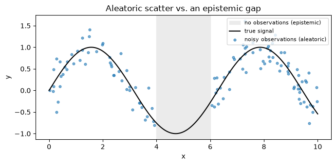
The vertical scatter of the points around the black curve is the aleatoric uncertainty: even with infinite data, single observations would still miss the curve by about the noise level. The shaded band is epistemic: the signal keeps oscillating there, but nothing in our data says so, and a model is free to do almost anything across the gap. Measuring inside the band would shrink that uncertainty; measuring more outside it would not.

Ways to add uncertainty to a neural network

In practice there are several ways to make a network produce a distribution instead of a point estimate (Haynes et al. 2023). None is universally best; they trade training cost, inference cost, and how much of the uncertainty they capture.

1. Learn the ensemble directly. Train one network to output \(K\) target values instead of one, so the model learns an ensemble prediction in a single forward pass. This needs ground truth ensembles (or a lot of data).

2. Multi-model ensembles. Train several independent networks that differ only in their random initialization (and the randomness of optimization). Their predictions disagree most where the data constrain them least, so the spread across members estimates epistemic uncertainty. This is often called a deep ensemble.

3. Predict distribution parameters. If the target is plausibly Gaussian, let the network output \(\mu\) and \(\sigma\) rather than \(y\); more complex parametric distributions work the same way.

4. Predict summary statistics. Instead of the parameters, output a set of quantiles of the target distribution.

5. Monte Carlo dropout. Dropout randomly zeroes a fraction of weights in each layer. During training this regularizes the model. If we keep dropout on during inference, every forward pass uses a slightly different subnetwork, so repeating the prediction many times yields a spread of outputs: uncertainty quantification almost for free.

Below we build a small deep ensemble (option 2) on the toy data: ten identical networks that differ only in random_state. To see where the members disagree, we also ask them to predict past \(x = 10\), beyond the last observation.

from sklearn.neural_network import MLPRegressor

X = x_obs.reshape(-1, 1)
ensemble = [
    MLPRegressor(hidden_layer_sizes=(50, 50), activation="relu",
                 max_iter=4000, random_state=s).fit(X, y_obs)
    for s in range(10)
]
xg = np.linspace(0, 14, 560)        # extends past the last observation at x = 10
preds = np.array([m.predict(xg.reshape(-1, 1)) for m in ensemble])
ens_mean, ens_spread = preds.mean(axis=0), preds.std(axis=0)

plt.figure(figsize=(7, 3.5))
plt.axvspan(4, 6, color="0.92")
plt.axvspan(10, 14, color="0.85")
plt.plot(xg, truth(xg), "k", lw=1.5, label="true signal")
plt.plot(xg, preds.T, color="tab:orange", lw=0.6, alpha=0.5)
plt.plot(xg, ens_mean, color="tab:red", lw=2, label="ensemble mean")
plt.fill_between(xg, ens_mean - 2 * ens_spread, ens_mean + 2 * ens_spread,
                 color="tab:red", alpha=0.15, label="mean ± 2 spread")
plt.scatter(x_obs, y_obs, s=8, alpha=0.4)
plt.xlabel("x"); plt.ylabel("y"); plt.legend(loc="upper left", fontsize=8)
plt.title("A deep ensemble: 10 networks, different initializations")
plt.tight_layout(); plt.show()

gap = (xg > 4) & (xg < 6)
beyond = xg > 10
data_region = ~gap & ~beyond
print(f"mean ensemble spread where we have data:  {ens_spread[data_region].mean():.3f}")
print(f"mean ensemble spread in the interior gap: {ens_spread[gap].mean():.3f}")
print(f"mean ensemble spread beyond x = 10:       {ens_spread[beyond].mean():.3f}")

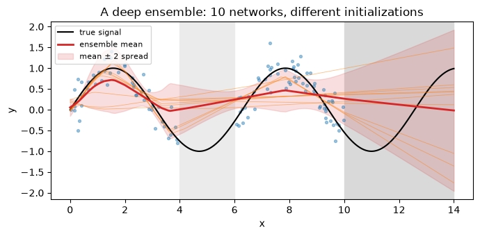
mean ensemble spread where we have data:  0.213
mean ensemble spread in the interior gap: 0.186
mean ensemble spread beyond x = 10:       0.635

Each thin orange line is one trained network. Beyond the edge of the data the members fan out dramatically, each extrapolating in its own direction, and the printed numbers confirm it: the spread past \(x = 10\) is about three times the spread over the observed region. The ensemble has discovered its own epistemic uncertainty there, without ever being told where the data end.

The interior gap teaches a subtler lesson. The members bridge it in nearly the same way, so the spread there is no larger than where we have data, even though the truth (which keeps oscillating) is far from all of them. With data on both sides, every network interpolates similarly and the ensemble stays confidently wrong. Deep ensembles reveal epistemic uncertainty most reliably under extrapolation; they can remain overconfident when interpolating across a gap, which is worth remembering whenever an ensemble looks reassuringly tight.

Evaluating predicted distributions: spread vs. skill

Once a model outputs distributions, evaluation has to change too. A first diagnostic borrowed from ensemble weather forecasting is the spread vs. skill plot:

• Spread is the uncertainty across ensemble members (their standard deviation).

• Skill is the accuracy of the ensemble mean (its absolute error).

For a well calibrated ensemble the two should match on average: when the ensemble claims a spread of 0.2, the mean should typically be wrong by about 0.2. Plotting binned skill against spread, a reliable ensemble follows the one-to-one line. Points above the line (error larger than spread) mean the ensemble is overconfident, or under-dispersive: it does not capture the true range of outcomes. Points below it mean the ensemble is underconfident. The plot answers two questions at once: does the ensemble capture the range of possible outcomes, and is the ensemble mean a reliable prediction?

An operational spread vs. skill plot aggregates over thousands of forecasts; here we only have the one toy problem, so we bin the 560 grid points by their ensemble spread and compare the average spread to the average error in each bin.

err = np.abs(ens_mean - truth(xg))

# bin points by ensemble spread and compare mean spread to mean error per bin
bins = np.quantile(ens_spread, np.linspace(0, 1, 9))
which = np.digitize(ens_spread, bins[1:-1])
bin_spread = np.array([ens_spread[which == b].mean() for b in range(8)])
bin_err = np.array([err[which == b].mean() for b in range(8)])

plt.figure(figsize=(4.5, 4.5))
lim = max(bin_spread.max(), bin_err.max()) * 1.1
plt.plot([0, lim], [0, lim], "k--", lw=1, label="perfect calibration")
plt.plot(bin_spread, bin_err, "o-", color="tab:red")
plt.xlabel("ensemble spread (binned)"); plt.ylabel("error of ensemble mean")
plt.title("Spread vs. skill"); plt.legend(fontsize=8)
plt.tight_layout(); plt.show()

print(f"correlation between spread and error: {np.corrcoef(ens_spread, err)[0, 1]:.2f}")

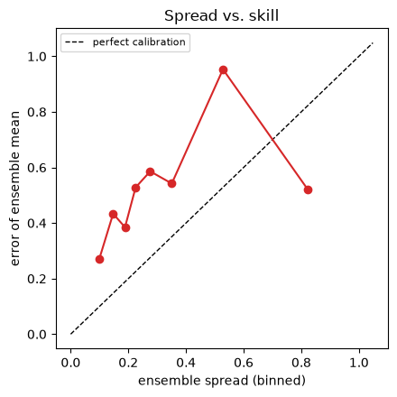
correlation between spread and error: 0.29

Through most of the range, bins with larger spread have larger error: spread is doing its job as a predictor of error. Two honest caveats are visible too. First, every bin sits above the one-to-one line, meaning the error is consistently larger than the spread claims: the ensemble is under-dispersive, or overconfident, a very common finding for deep ensembles, whose members (differing only in initialization) rarely fan out as widely as the true range of possibilities. Second, the largest spread bin breaks the trend: at extreme extrapolation the members fan out so symmetrically that their mean lands near the middle by construction, and with a single toy realization these statistics are noisy anyway. Diagnostics like this one are only trustworthy when averaged over many cases.

The continuous ranked probability score

Spread vs. skill diagnoses calibration, but we also want a single score to compare probabilistic models, the way MAE or MSE compares deterministic ones. The standard choice is the continuous ranked probability score:

\[\mathrm{CRPS}(F, y) = \int_{-\infty}^{\infty} \left( F(z) - \mathbb{1}\{z \ge y\} \right)^2 \, dz\]

where \(F\) is the forecast’s cumulative distribution function (CDF) and \(y\) is the observed value. Graphically: draw the forecast CDF, draw the step function that jumps from 0 to 1 at the observation, and add up the squared area between them. A sharp forecast centered on the observation makes that area small, so lower CRPS is better. If the forecast is a single deterministic value, its CDF is itself a step function and the CRPS reduces exactly to the mean absolute error, which is what makes it a genuine generalization of the deterministic metrics we already use.

def crps_from_samples(samples, y, zgrid):
    "CRPS of an empirical (ensemble) forecast, by numerical integration."
    F = (np.sort(samples)[:, None] <= zgrid[None, :]).mean(axis=0)
    H = (zgrid >= y).astype(float)
    return np.trapz((F - H) ** 2, zgrid)

# evaluate at one point beyond the data, where the members disagree
x0 = 12.0
i0 = np.argmin(np.abs(xg - x0))
members = preds[:, i0]
y0 = truth(x0)
zg = np.linspace(-5, 5, 4001)

F = (np.sort(members)[:, None] <= zg[None, :]).mean(axis=0)
H = (zg >= y0).astype(float)

plt.figure(figsize=(6, 3.5))
plt.plot(zg, F, label="forecast CDF (ensemble)")
plt.plot(zg, H, "k", label="observation (step)")
plt.fill_between(zg, F, H, alpha=0.2, label="area that CRPS penalizes")
plt.xlim(-2.5, 2.5); plt.xlabel("z"); plt.ylabel("cumulative probability")
plt.title(f"CRPS at x = {x0}"); plt.legend(fontsize=8)
plt.tight_layout(); plt.show()

crps_ens = crps_from_samples(members, y0, zg)
det = members[0]                       # a single deterministic forecast
crps_det = crps_from_samples(np.array([det]), y0, zg)
print(f"observation y = {y0:.3f}")
print(f"CRPS of the 10-member ensemble:      {crps_ens:.3f}")
print(f"CRPS of a single member:             {crps_det:.3f}")
print(f"|error| of that member (MAE check):  {abs(det - y0):.3f}")

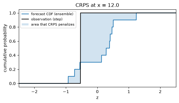
observation y = -0.537
CRPS of the 10-member ensemble:      0.436
CRPS of a single member:             0.817
|error| of that member (MAE check):  0.817

The printed numbers make both claims of the previous section concrete. First, the CRPS of the single deterministic member equals its absolute error (up to the resolution of the integration grid): CRPS really does reduce to MAE in the deterministic case. Second, at this point beyond the data, where the members genuinely disagree, the ensemble scores markedly better than the single member: spreading probability over the plausible range is rewarded when any one point prediction is likely to be off.

Summary

• Generative models predict distributions of outputs rather than single vectors, which lets them express uncertainty instead of hiding it.

• Aleatoric uncertainty is irreducible scatter; epistemic uncertainty reflects missing data and can be reduced by observing more.

• Practical routes to uncertainty: learned ensembles, deep ensembles, predicted distribution parameters, predicted quantiles, and Monte Carlo dropout.

• Evaluate probabilistic predictions with spread vs. skill for calibration and CRPS for scoring; CRPS generalizes MAE.

The next page introduces the first two of three state-of-the-art generative architectures: generative adversarial networks and diffusion models.