
Recurrent Neural Networks and Time Series#
The artificial neural network makes no assumption about how its inputs are arranged, and the convolutional neural network builds in a spatial inductive bias for images and gridded fields. This section introduces the third major architecture: the recurrent neural network (RNN), a regularized neural network built to process sequences, above all the time series that fill environmental science. We will:
Define the recurrent neural network and distinguish it from the CNN.
Discuss forecasting in the context of environmental time series.
Define natural language processing, where these architectures originated.
Understand several ML architectures used for time series prediction: the vanilla RNN, the LSTM, the GRU, and (briefly) the transformer.
Discuss inductive bias in machine learning models.
import numpy as np
import matplotlib.pyplot as plt

rng = np.random.default_rng(0)
From images to sequences#
A fully connected neural network can learn a mapping from any set of input features to an output, but it shares no weights and assumes no structure. The CNN regularizes it for spatial data by sliding one small filter across the whole map. The RNN applies the same trick along a different axis: it is a regularized neural network for sequences, sharing one set of weights across every time step instead of every pixel.
RNNs were originally developed for natural language processing (NLP), the subset of artificial intelligence focused on using machines to interpret and understand human language. A sentence is a sequence of words, and a canonical NLP task is: given the first few words, predict the next one. The same machinery powers:
Speech recognition: map a sound wave to the words it contains, the basis of voice assistants like Siri or Alexa.
Machine translation: translate a sentence between languages, hard because word order differs and there is rarely a one-to-one mapping between words.
RNNs in environmental science#
In climate and environmental applications we mostly use these architectures for time series prediction: modeling how an environmental system changes over time.
Rainfall-runoff modeling in hydrology. Predict the discharge of a stream from meteorological forcing. This is hard to do with a numerical model: flooding depends not just on today’s precipitation but on the past precipitation, the topography of the catchment, snowpack, and more. Large community datasets (CAMELS, with 35 years of daily forcing and discharge for 671 US basins, and its global successor Caravan) have enabled so-called catchment-independent rainfall-runoff models trained across many streams at once.
Dynamic time series modeling. Predict a quantity like humidity that has a diurnal cycle with weather-driven variability on top.
Dynamic land cover classification. Combine sequential models with CNNs to track how land cover changes over time from satellite imagery.
Four ways to set up a forecast#
The same recurrent machinery supports several problem setups, and choosing one is the first modeling decision:
Sequence to sequence: features at every time step in, a prediction at every time step out (e.g. meteorology in, water level out, day by day).
Sequence to vector: several past time steps in, a single prediction out. The rainfall-runoff example in the companion tutorial works this way: the previous 365 days of meteorology predict today’s discharge.
Vector to sequence: one set of input features in, a sequence of future values out.
Encoder-decoder: an encoder network compresses the input sequence into a learned latent representation (an encoding), and a separate decoder network unrolls that representation into the output sequence. This split appears all over machine learning and is useful when the output is a related but different variable from the input.
Windowing: reshaping a time series into training samples#
Whichever setup we choose, the raw data is one long continuous series, and the model expects samples of shape (sequence length, number of features). We build them by sliding a window along the series. Here is the idea on a toy series, with a sequence length of three:
series = np.arange(6)          # a toy "time series": 0, 1, 2, 3, 4, 5
seq_len = 3

X = np.array([series[i:i + seq_len] for i in range(len(series) - seq_len)])
y = series[seq_len:]

for inputs, target in zip(X, y):
    print(f"input window {inputs} -> target {target}")
input window [0 1 2] -> target 3
input window [1 2 3] -> target 4
input window [2 3 4] -> target 5
Each input window carries its own short history, and the targets start
seq_len points into the series: the first three values have no complete
window before them, so the first target is the fourth value. Lining the
targets up this way is easy to get wrong and important to check. Deep learning
libraries provide utilities for exactly this reshaping (in TensorFlow,
tf.keras.utils.timeseries_dataset_from_array).
One practical note: because every window already contains its own history, the training windows can be shuffled freely during training. But when evaluating on a test period we keep the windows in temporal order, so the predicted series can be compared against the observed one.
The baseline to beat: persistence#
Why is naive forecasting (also called persistence forecasting), which simply predicts that the next value equals the current one, so hard to outperform? Because environmental time series usually have strong autocorrelation in time: if the sun rose yesterday, it will probably rise today. Any model worth training has to beat this near-free baseline.
We can see this on a synthetic hourly “humidity” series with a diurnal cycle plus slowly varying (red) noise:
hours = np.arange(24 * 60)                       # 60 days, hourly
diurnal = 15 * np.sin(2 * np.pi * hours / 24)    # daily cycle
red = np.zeros(len(hours))                       # slowly varying noise
for t in range(1, len(hours)):
    red[t] = 0.95 * red[t - 1] + rng.normal(0, 2)
humidity = 60 + diurnal + red

r1 = np.corrcoef(humidity[:-1], humidity[1:])[0, 1]
mae_persistence = np.mean(np.abs(humidity[1:] - humidity[:-1]))
mae_climatology = np.mean(np.abs(humidity - humidity.mean()))

print(f"lag-1 autocorrelation      : {r1:.3f}")
print(f"persistence forecast MAE   : {mae_persistence:.2f}")
print(f"climatology (mean) MAE     : {mae_climatology:.2f}")

fig, ax = plt.subplots(1, 2, figsize=(10, 3.5))
ax[0].plot(hours[:240] / 24, humidity[:240])
ax[0].set_xlabel("day"); ax[0].set_ylabel("relative humidity (%)")
ax[0].set_title("synthetic humidity, first 10 days")
ax[1].scatter(humidity[:-1], humidity[1:], s=2, alpha=0.3)
ax[1].set_xlabel("value at hour t"); ax[1].set_ylabel("value at hour t+1")
ax[1].set_title(f"lag-1 autocorrelation r = {r1:.2f}")
plt.tight_layout(); plt.show()
lag-1 autocorrelation      : 0.962
persistence forecast MAE   : 2.89
climatology (mean) MAE     : 10.55
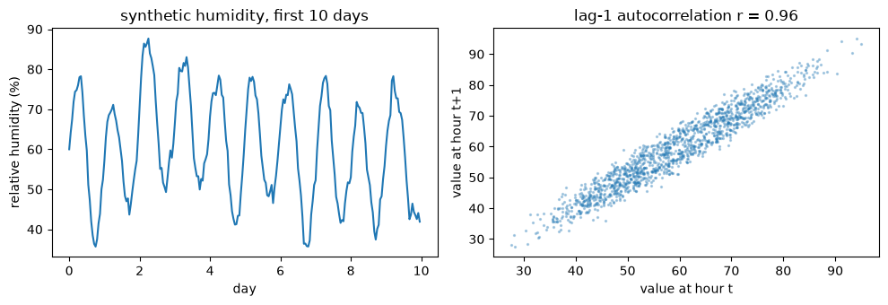
Consecutive hours are almost identical (the lag-1 scatter hugs the diagonal), so just repeating the last value is several times more accurate than predicting the long-term mean. A model that fails to beat persistence has effectively learned nothing beyond “tomorrow looks like today.”
We saw in the CNN section that a 1-D convolution can also process a time series by sliding a fixed kernel of weights along the signal. It is simple and inexpensive, but the kernel only ever sees a fixed-width window: it carries no memory of what happened before it. For time series prediction, recurrent architectures generally work better.
Algorithms to process time series#
We will look at four architectures, in the order they were developed: the vanilla RNN, the long short-term memory (LSTM), the gated recurrent unit (GRU), and the transformer. (“Vanilla” is machine learning slang for the plain, original variant of a model, without extra complications.)
The vanilla RNN#
The regularization idea: use the same update rule, with the same weights, at every time step. At step \(t\) the network takes the current input vector \(\mathbf{x}_t\) and the previous hidden state \(\mathbf{h}_{t-1}\), and produces a new hidden state:
If we want a prediction at step \(t\), another layer maps the hidden state to the output (followed by a softmax for classification, or nothing extra for regression):
Because \(\mathbf{W}_h\), \(\mathbf{W}_x\), and \(\mathbf{b}\) are shared across all time steps, the RNN is effectively learning a single model that it applies at every step. This is exactly what a physical model does: the physics of the system does not change from one time step to the next, only the state does.
Why the hyperbolic tangent? The \(\tanh\) activation bounds each component of the hidden state between \(-1\) and \(1\). An unbounded activation like ReLU (which ranges from 0 to infinity) can let the hidden state grow without limit as it is fed back through the recurrence step after step, the exploding regime. The demo below runs the same recurrence with the same weight matrix under both activations:
n_hidden, n_steps = 10, 60
W = rng.normal(0, 1, (n_hidden, n_hidden))
W *= 2.0 / np.max(np.abs(np.linalg.eigvals(W)))   # fix the spectral radius at 2

inputs = rng.normal(0, 0.5, (n_steps, n_hidden))

def run_recurrence(activation):
    h, norms = np.zeros(n_hidden), []
    for x in inputs:
        h = activation(W @ h + x)
        norms.append(np.linalg.norm(h))
    return np.array(norms)

tanh_norms = run_recurrence(np.tanh)
relu_norms = run_recurrence(lambda z: np.maximum(z, 0))

print(f"tanh: final hidden-state norm {tanh_norms[-1]:.2f} "
      f"(bound: sqrt({n_hidden}) = {np.sqrt(n_hidden):.2f})")
print(f"relu: final hidden-state norm {relu_norms[-1]:.2e}")

plt.figure(figsize=(6, 3.5))
plt.semilogy(tanh_norms, label="tanh")
plt.semilogy(relu_norms, label="ReLU")
plt.xlabel("time step"); plt.ylabel("|| hidden state ||")
plt.title("the same recurrence with two activations")
plt.legend(); plt.tight_layout(); plt.show()
tanh: final hidden-state norm 2.40 (bound: sqrt(10) = 3.16)
relu: final hidden-state norm 4.21e+03
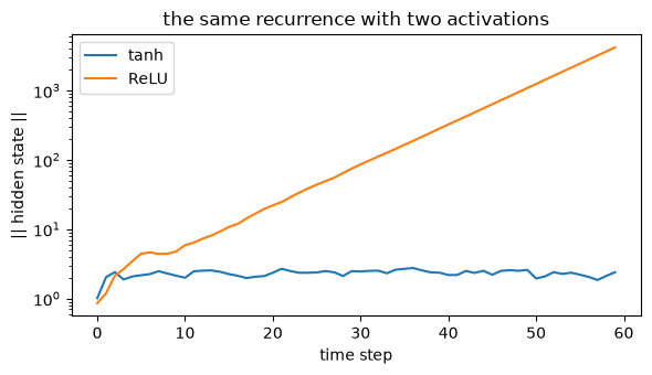
With identical weights, the ReLU hidden state grows by orders of magnitude over 60 steps while the tanh hidden state stays bounded (its norm can never exceed \(\sqrt{10} \approx 3.2\) for 10 hidden units, since every component lies in \([-1, 1]\)). This is why recurrent architectures use tanh.
The short-term memory problem#
The price of the recurrence is that vanilla RNNs forget: they represent the recent past well but gradually lose information about earlier inputs. An environmental system can have correlations on many timescales at once (daily, seasonal, yearly), and a model that only remembers the last few steps will miss the longer ones.
We can measure the forgetting directly: run the same input sequence twice, perturb only the first input, and watch how long the difference between the two hidden-state trajectories survives:
W_mem = rng.normal(0, 1, (n_hidden, n_hidden))
W_mem *= 0.9 / np.max(np.abs(np.linalg.eigvals(W_mem)))  # stable regime

inputs_mem = rng.normal(0, 0.5, (n_steps, n_hidden))

def run_sequence(xs):
    h, states = np.zeros(n_hidden), []
    for x in xs:
        h = np.tanh(W_mem @ h + x)
        states.append(h.copy())
    return np.array(states)

perturbed = inputs_mem.copy()
perturbed[0] += 1.0                       # change only the first input

diff = np.linalg.norm(run_sequence(perturbed) - run_sequence(inputs_mem), axis=1)
for step in (0, 9, 29, 59):
    print(f"effect of the perturbation after step {step + 1:2d}: {diff[step]:.1e}")

plt.figure(figsize=(6, 3.5))
plt.semilogy(np.arange(1, n_steps + 1), diff)
plt.xlabel("time step")
plt.ylabel("|| difference in hidden state ||")
plt.title("how long the first input is remembered")
plt.tight_layout(); plt.show()
effect of the perturbation after step  1: 2.1e+00
effect of the perturbation after step 10: 1.1e-01
effect of the perturbation after step 30: 5.1e-05
effect of the perturbation after step 60: 4.7e-09
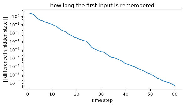
The influence of the first input decays roughly exponentially: within a few dozen steps it is smaller than any signal the network could use. For a 365-day input sequence, a vanilla RNN will do a much better job representing last week’s rainfall than last winter’s snowpack.
Long short-term memory (LSTM)#
The LSTM is a more advanced recurrent architecture designed to handle longer-range dependencies. It tackles the short-term memory problem by carrying two states forward:
the usual hidden state \(\mathbf{h}_t\), tracking the immediate past, and
a cell state \(\mathbf{c}_t\), a longer-term memory that changes only slowly from step to step.
Traffic between the two is managed by three gates, each of which is itself a small neural network (with its own weights) applied to the concatenation of the previous hidden state and the current input:
The candidate update is a tanh layer, and the gates decide what the cell state drops, what it writes, and what it exposes:
The forget gate decides which parts of the long-term memory to erase, the input gate decides which parts of the new candidate to write, and the output gate decides how much of the cell state shows up in the hidden state. Because the cell state is updated additively (a gated copy of itself plus a gated new term) rather than being squashed through the recurrence at every step, information can survive across many more time steps than in the vanilla RNN. A typical application: modeling air quality in a city, where the prediction depends on traffic, weather, and emissions over multiple timescales.
Gated recurrent unit (GRU)#
The GRU came after the LSTM and simplifies it, asking whether all that machinery is really needed:
a single state vector \(\mathbf{h}_t\) (no separate cell state),
a single gate controller \(\mathbf{z}_t\) that handles both forgetting and writing (whatever is forgotten is replaced by new content),
no output gate, just a reset gate \(\mathbf{r}_t\) that controls how much of the previous state feeds into the candidate update.
It is used for the same tasks: predicting river flow rates from rainfall, snowmelt, and temperature, for instance, where the gating helps capture the complex dependencies.
Which one to use?#
In practice you would try the RNN and the LSTM on the same problems. The LSTM generally works a little better because it can track dependencies on several timescales, while the vanilla RNN forgets. But if the distant past genuinely matters little for your problem, the simpler RNN, with far fewer weights to learn, can do as well or better. The GRU sits in between. For the same hidden size, the parameter counts differ by the number of internal networks each architecture carries:
n_h, n_features = 10, 5      # hidden units, input features per time step

per_network = n_h * (n_h + n_features) + n_h   # weights (recurrent + input) + biases
for name, n_networks in [("vanilla RNN", 1), ("GRU", 3), ("LSTM", 4)]:
    print(f"{name:12s}: {n_networks} internal network(s) x {per_network} "
          f"= {n_networks * per_network:4d} parameters")
vanilla RNN : 1 internal network(s) x 160 =  160 parameters
GRU         : 3 internal network(s) x 160 =  480 parameters
LSTM        : 4 internal network(s) x 160 =  640 parameters
With 10 hidden units and 5 input features, one recurrent layer costs 160 parameters as a vanilla RNN, 480 as a GRU (three internal networks: reset gate, update gate, candidate), and 640 as an LSTM (four: three gates plus the candidate). All three then need the same small dense layer to map the final hidden state to the prediction. More capacity to remember costs more weights to learn, which is the trade-off to weigh against how much training data you have.
Attention and transformers#
Most of the recent innovation in sequence modeling has gone into the attention mechanism. The motivation came from machine translation: translating a sentence is not a word-by-word lookup, because word order differs between languages and several words of context may determine how one word should be translated. Rather than stepping through the sequence one element at a time, attention lets the model look at the entire sequence at once and learn which parts to pay attention to for the prediction at hand.
Formally, attention is an interface between an encoder and a decoder that provides information about every encoder hidden state. The recipe:
Prepare hidden states. Run the encoder over the input sequence to get a hidden state for every element.
Score every encoder hidden state against the current decoder state (this small learned network is called the alignment model).
Softmax the scores, so they become positive weights that sum to 1.
Weight each encoder hidden state by its softmaxed score.
Sum the weighted states into a single context vector.
Feed the context vector into the decoder, which produces the output.
Every weight involved is learned by the same gradient descent as the rest of the network. Here is the entire mechanism in a few lines of numpy, for a toy sequence of four encoder states scored against one decoder state:
encoder_states = np.array([[1.0, 0.0],     # 4 encoder hidden states,
                           [0.8, 0.6],     # 2 dimensions each
                           [0.0, 1.0],
                           [-0.5, 0.5]])
decoder_state = np.array([0.9, 0.4])

scores = encoder_states @ decoder_state          # step 2: score each state
weights = np.exp(scores) / np.exp(scores).sum()  # step 3: softmax
context = weights @ encoder_states               # steps 4 + 5: weight and sum

print("scores           :", np.round(scores, 2))
print("attention weights:", np.round(weights, 3), " (sum =", weights.sum(), ")")
print("context vector   :", np.round(context, 3))

plt.figure(figsize=(5, 3))
plt.bar(range(len(weights)), weights)
plt.xticks(range(len(weights)), [f"state {i}" for i in range(len(weights))])
plt.ylabel("attention weight")
plt.title("how much the decoder attends to each encoder state")
plt.tight_layout(); plt.show()
scores           : [ 0.9   0.96  0.4  -0.25]
attention weights: [0.335 0.356 0.203 0.106]  (sum = 1.0 )
context vector   : [0.567 0.47 ]
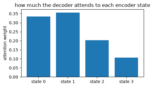
The two encoder states most similar to the decoder state get the largest weights, and the context vector is pulled toward them; the weights sum to exactly 1. In a trained model the scoring is done by a learned alignment network rather than a raw dot product, but the flow is the same.
Transformers stack these attention layers into a full encoder-decoder architecture, dispensing with recurrence entirely. Introduced around 2017, transformers have revolutionized neural machine translation (using ML to predict the likelihood of a sequence of words) and are the architecture behind large language models: GPT stands for generative pretrained transformer. A nice interactive visualization of a transformer-based LLM is at https://bbycroft.net/llm. For environmental time series, though, transformers are not automatically the best choice: the more traditional RNNs, LSTMs, and GRUs remain very useful.
Graph neural networks#
Not all data is a grid or a sequence. Graph neural networks (GNNs) are deep learning architectures for graph-structured data: a set of nodes, each with its own feature vector, connected by edges that encode arbitrary relationships. We only touch on them here so you know they exist. With a GNN you can make predictions at the node level (given a node’s connectivity), predict how nodes should be linked, or classify whole graphs.
Two climate examples:
GraphCast, an ML-based numerical weather prediction model, treats each latitude, longitude, and height point as a node in a graph and adds nested graphs at multiple resolutions, so the model can capture not just local structure but long-range connectivity (the jet stream, or a sea surface temperature change in one basin affecting weather elsewhere). It performs on par with state-of-the-art numerical weather prediction.
Sparse sensor networks: with air quality sensors scattered irregularly over a city, a GNN can learn spatial relationships between sites, so a prediction at one site can borrow information from its neighbors.
Inductive bias in machine learning models#
We can now line up all the deep learning architectures of this unit by the assumption each one builds in:
Data |
Architecture |
Inductive bias |
|---|---|---|
Tabular features |
Fully connected ANN |
None: any input can relate to any output |
Images, spatial maps |
CNN |
Spatial translation invariance: weights shared across space |
Sequences, time series |
RNN / LSTM / GRU |
Time translation invariance: weights shared across time steps |
Graphs, unstructured meshes |
GNN |
Relational: nodes treated according to their connectivity |
Choosing the architecture whose inductive bias matches the problem can significantly reduce the amount of training data needed and improve predictive skill. A recurrent model applied to a sequential task will beat a fully connected network with many more weights, because the fully connected network has to learn the structure the recurrent model gets for free.
These building blocks also combine. A CNN can encode each frame of a spatial field into a hidden state that an LSTM then evolves through time (CNN-LSTM, for spatio-temporal prediction such as forecasting how a map of a variable changes). A GNN can do the same for sparse sensor sites, with an LSTM handling the time dimension (GNN-LSTM, for time series prediction on unstructured meshes). Picking an inductive bias is where our physical intuition about a problem enters the architecture itself.