
Convolutional Neural Networks#
The artificial neural network of the previous section is a fully connected model: every input connects to every neuron in the next layer. That is a lot of freedom, and for spatial data (images, and gridded climate fields), most of it is wasted. This section introduces the convolutional neural network (CNN), a regularized neural network built specifically to process images and any data with spatial structure. We will:
Define the convolutional neural network and see where its efficiency comes from.
Survey the main applications of CNNs, in computer vision and in climate and environmental research.
Walk through the operations that make up a CNN (convolution, stride, pooling, padding) and the steps to design and train one.
Define transfer learning and understand how to reuse pre-trained models.
As with the ANN page, every figure below is generated from a few lines of numpy
and one of scikit-learn’s bundled toy images, so you can watch each operation happen
rather than take it on faith.
import numpy as np
import matplotlib.pyplot as plt
from sklearn.datasets import load_digits

np.random.seed(0)
From a fully connected network to a convolution#
A fully connected (feed-forward, multilayer-perceptron) network makes no assumption about how its inputs are arranged: pixel (0, 0) and pixel (95, 143) are treated as interchangeable coordinates in one long vector. But in an image, pixels that are spatially close carry related information: an edge, a texture, a storm front. A CNN builds this in as a spatial inductive bias: instead of one weight per input–output pair, it learns a small filter (also called a kernel) of weights and slides it across the image, reusing the same weights at every location.
This is the “regularized neural network” idea: weight sharing dramatically reduces the number of parameters and forces the network to look for local patterns that are useful anywhere in the image. (In the next class we will meet recurrent neural networks, which encode a different inductive bias, one for sequential data such as time series, but the CNN’s bias is spatial.)
What CNNs are used for#
CNNs grew out of computer vision: using machine learning to analyze images and videos (a video being a sequence of images). A few canonical tasks, each of which asks a different question of the same picture:
Classification: what is in the image? (cat vs. dog)
Classification + localization: what, and where is the single object?
Semantic segmentation: label every pixel by class (grass, cat, sky, tree). It classifies pixels, not objects, so it tells you where a class is but not how many.
Object detection / instance segmentation: find multiple objects and separate them (three dogs, and which pixels belong to each).
In remote sensing and climate#
These tasks are enormously useful for remote sensing, where we now hold terabytes to petabytes of satellite imagery. A CNN can sweep through it far faster than any human:
Object detection: locate every airplane on an airport apron, or map every solar panel on Earth for downstream energy studies.
Instance segmentation for storm detection: a storm system is not a neatly defined variable in a climate model, but a CNN can be trained to outline where tropical cyclones and atmospheric rivers sit in a model field. Run that over ~100 years of model output and you get storm counts and locations that would be impractical to extract by hand.
Contrails and aviation climate effects: contrails are high-altitude cirrus clouds that form from aircraft exhaust; in the right conditions they trap outgoing longwave radiation, a warming (positive) forcing in the same direction as CO₂. Recent work suggests contrails may contribute more than 60% of aviation’s climate forcing, more than the CO₂ from the fuel itself. Whether a given flight makes a long-lived contrail is very hard to model, so groups such as Google’s Project Contrails hand-label contrail masks in GOES-16 satellite imagery and train CNNs to detect them, then apply the model back to the full satellite record.
Other environmental applications: classify a catchment as flooded or not, label a scene as forest / non-forest, outline individual rock glaciers, or identify every tree in an image (and monitor all of these over time).
A climate-model field can be treated like an image, though it may have many more channels than an ordinary picture, which brings us to how the convolution actually works.
The convolution operation#
One dimension first#
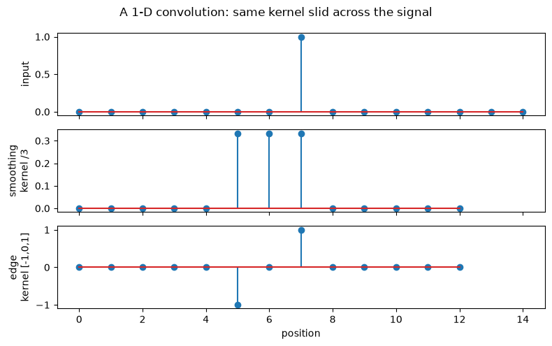
The simplest case is a 1-D convolution. We have a short kernel of learnable weights and a longer signal. We slide the kernel along the signal and, at each position, output the weighted sum of the input value and its neighbours. It is simple and computationally inexpensive.
Below, the signal is mostly zeros with a single spike. Convolving it with a small
averaging kernel spreads the spike over its neighbours; convolving with an
edge-detection kernel [-1, 0, 1] responds only where the signal changes. The
weights shown here are fixed for illustration. In a real CNN these are exactly the
numbers the network learns during training.
def conv1d(signal, kernel):
    # 'valid' 1-D convolution: slide the (flipped) kernel over the signal
    k = kernel[::-1]
    out = np.array([np.dot(signal[i:i+len(k)], k)
                    for i in range(len(signal) - len(k) + 1)])
    return out

signal = np.zeros(15); signal[7] = 1.0            # a single spike
smooth = np.array([1, 1, 1]) / 3.0                # local average
edge   = np.array([-1, 0, 1])                      # responds to change

print("input signal :", signal.astype(int))
print("smoothed     :", np.round(conv1d(signal, smooth), 2))
print("edge-filtered:", conv1d(signal, edge).astype(int))

fig, ax = plt.subplots(3, 1, figsize=(8, 5), sharex=True)
ax[0].stem(signal); ax[0].set_ylabel("input")
ax[1].stem(conv1d(signal, smooth)); ax[1].set_ylabel("smoothing\nkernel /3")
ax[2].stem(conv1d(signal, edge)); ax[2].set_ylabel("edge\nkernel [-1,0,1]")
ax[2].set_xlabel("position")
fig.suptitle("A 1-D convolution: same kernel slid across the signal")
plt.tight_layout(); plt.show()
input signal : [0 0 0 0 0 0 0 1 0 0 0 0 0 0 0]
smoothed     : [0.   0.   0.   0.   0.   0.33 0.33 0.33 0.   0.   0.   0.   0.  ]
edge-filtered: [ 0  0  0  0  0 -1  0  1  0  0  0  0  0]
Two dimensions#
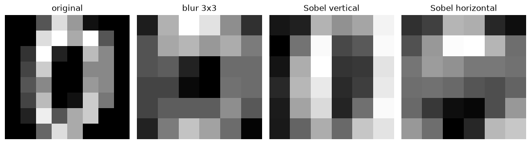
For images we slide a 2-D kernel (often a small 3×3 receptive field) across the array. At each location the kernel’s weights multiply the pixels underneath and are summed to a single output value; the result is a convolved feature map that becomes the input to the next layer.
Different kernels extract different features. Below we take one handwritten digit from
scikit-learn’s bundled load_digits (an 8×8 grayscale image) and pass a blur
kernel and two edge-detection (Sobel) kernels over it. The blur smooths; the Sobel
kernels light up vertical and horizontal edges respectively. A trained CNN
learns a whole bank of such kernels automatically.
def conv2d(img, kernel):
    # 'valid' 2-D convolution (correlation with a flipped kernel), plain numpy
    k = kernel[::-1, ::-1]
    kh, kw = k.shape
    H, W = img.shape
    out = np.zeros((H - kh + 1, W - kw + 1))
    for i in range(out.shape[0]):
        for j in range(out.shape[1]):
            out[i, j] = np.sum(img[i:i+kh, j:j+kw] * k)
    return out

img = load_digits().images[0]                      # one 8x8 digit

blur      = np.ones((3, 3)) / 9.0
sobel_v   = np.array([[-1, 0, 1], [-2, 0, 2], [-1, 0, 1]])   # vertical edges
sobel_h   = sobel_v.T                                         # horizontal edges

fig, ax = plt.subplots(1, 4, figsize=(11, 3))
for a, (title, out) in zip(ax, [
        ("original", img),
        ("blur 3x3", conv2d(img, blur)),
        ("Sobel vertical", conv2d(img, sobel_v)),
        ("Sobel horizontal", conv2d(img, sobel_h))]):
    a.imshow(out, cmap="gray"); a.set_title(title); a.axis("off")
plt.tight_layout(); plt.show()
Multiple channels#
A colour image is not a single array but three channels: red, green, blue. A convolutional layer handles this by giving each kernel a depth matching the input, then summing over the channels (as well as over height and width) to produce each output value. A layer also learns not one but many filters, so its output has as many channels as it has filters. Climate-model fields work the same way, often with many more than three channels (temperature, humidity, winds at many levels).
Stride: moving the filter in bigger steps#
The stride is how far the filter moves at each step. A stride of 1 visits every position (as above). A larger stride skips positions, producing fewer outputs and therefore a smaller feature map than the input.
Why shrink on purpose? For a task like classification we want to funnel a 128×128 image down to a single class probability (a softmax over classes), so reducing spatial size as we go deeper is exactly what we want.
def conv2d_stride(img, kernel, stride):
    k = kernel[::-1, ::-1]; kh, kw = k.shape; H, W = img.shape
    rows = range(0, H - kh + 1, stride); cols = range(0, W - kw + 1, stride)
    return np.array([[np.sum(img[i:i+kh, j:j+kw] * k) for j in cols] for i in rows])

img16 = load_digits().images[0]   # 8x8
for s in (1, 2, 3):
    out = conv2d_stride(img16, blur, stride=s)
    print(f"stride {s}: 8x8 input, 3x3 kernel  ->  output {out.shape}")
stride 1: 8x8 input, 3x3 kernel  ->  output (6, 6)
stride 2: 8x8 input, 3x3 kernel  ->  output (3, 3)
stride 3: 8x8 input, 3x3 kernel  ->  output (2, 2)
Pooling: shrinking without weights#
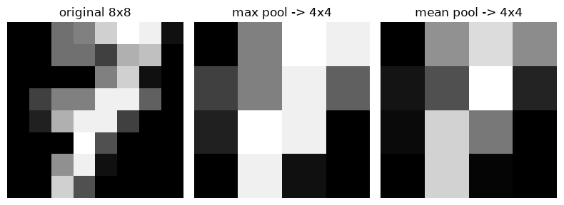
Another way to shrink a feature map is a pooling layer. Unlike a convolution, pooling has no learnable weights; it just summarizes each little patch. Max pooling keeps the largest value in each 2×2 block; average (mean) pooling keeps the mean. A 2×2 pool turns four pixels into one, compressing the image by a factor of four while keeping its overall structure.
def pool2x2(img, mode="max"):
    H, W = img.shape; H -= H % 2; W -= W % 2      # trim to even size
    blocks = img[:H, :W].reshape(H // 2, 2, W // 2, 2)
    return blocks.max((1, 3)) if mode == "max" else blocks.mean((1, 3))

img8 = load_digits().images[7]
fig, ax = plt.subplots(1, 3, figsize=(8, 3))
for a, (title, out) in zip(ax, [("original 8x8", img8),
                                ("max pool -> 4x4", pool2x2(img8, "max")),
                                ("mean pool -> 4x4", pool2x2(img8, "mean"))]):
    a.imshow(out, cmap="gray"); a.set_title(title); a.axis("off")
print("original:", img8.shape, " pooled:", pool2x2(img8).shape)
plt.tight_layout(); plt.show()
original: (8, 8) pooled: (4, 4)
Building a convolutional neural network#
Put these pieces together and a typical CNN looks like:
Prepare and load the image dataset.
A series of convolution and pooling layers, which progressively extract higher-level features while shrinking the spatial size.
A flatten layer that turns the final 2-D feature maps into a single vector.
A few dense (fully connected) layers, the same kind as in the ANN, ending, for classification, in a softmax over classes.
CNNs expose even more hyperparameters than a plain neural network (kernel size, number of filters, stride, pooling, how many conv/pool blocks), so architecture design is, again, “more art than science,” guided by rules of thumb and problem-specific experience rather than one correct answer.
Not enough data? Augment it#
CNNs typically need more data than a plain neural network to train well. When you only have, say, 1000 images, data augmentation generates realistic variants of each training image (rotations, translations, resizing, colour shifts), so a cat is recognized at any size or position. Deep-learning libraries (TensorFlow/Keras) provide these transforms ready-made. As a bonus, augmentation regularizes the model, helping it generalize to new images.
Padding: keeping the size fixed#
Each convolution shrinks the image at the edges (a 3×3 kernel loses a one-pixel
border). When you want the output to stay the same size as the input, use zero
padding: ring the image with zeros so the kernel has something to sit on at the edge.
In Keras this is the difference between padding="same" (pad to preserve size) and
padding="valid" (no padding, let the image shrink).
def pad_same(img, k=3):
    p = k // 2
    return np.pad(img, p, mode="constant")

img8 = load_digits().images[0]
print("valid (no padding): 8x8 in ->", conv2d(img8, blur).shape, "  (shrinks)")
print("same  (zero-pad)  : 8x8 in ->", conv2d(pad_same(img8, 3), blur).shape, "  (preserved)")
valid (no padding): 8x8 in -> (6, 6)   (shrinks)
same  (zero-pad)  : 8x8 in -> (8, 8)   (preserved)
A note on batch size and hardware#
CNNs are usually trained on GPUs, which are fast but have limited memory (RAM). A large batch of high-resolution images may not fit, so we train on smaller batches (a subset of the data at a time), as both a memory necessity and, via stochastic gradient descent, a route to a more generalizable solution. Reducing batch size, using fewer layers, or increasing strides all lower memory use.
Transfer learning#
Sometimes even with augmentation there is still not enough data to train a good CNN from scratch. Transfer learning reuses a model already trained on a large dataset for a different problem.
When computer vision took off in the early 2010s, the community built huge labelled benchmark datasets (most famously ImageNet) and trained strong architectures on them (ResNet, U-Net, and others). A network trained on millions of images has learned, in its convolutional layers, a hierarchy of higher-level features (edges, textures, shapes) that turn out to be useful for almost any vision task. So instead of starting from random weights, we:
Pick a pre-trained model to reuse (e.g. ResNet).
Load its trained weights, corresponding to a similar dataset.
Retrain only part of it: typically freeze most layers and retrain just the final few dense layers (or the first layers closest to the image, which are most specialized to the new input), keeping the general features the rest already learned.
These pre-trained models load directly from libraries like TensorFlow/Keras.
CNNs and transfer learning in climate science#
The same ideas transfer to climate problems, where the recurring question is: how do we emulate a complex, high-dimensional, spatial environmental process cheaply?
Spatial emulation. Because a climate-model field is image-like, a CNN can learn to map inputs (e.g. greenhouse-gas concentrations) to a full 2-D temperature map, and, unlike a plain neural network, it can predict that map directly without flattening away the spatial structure. The companion tutorial does exactly this on the ClimateBench dataset (surface-temperature maps from the NorESM2 model driven by greenhouse-gas concentrations under different SSP scenarios), comparing a dense network against a CNN, which needs no flattening step and reaches comparable accuracy with fewer weights.
Reducing uncertainty in climate projections via transfer learning. Projections of future surface temperature spread widely by 2100, roughly 2 °C to 4.5 °C across models under a given scenario, because different models parameterize the physics differently. We have many climate models but only one observed Earth. A recent approach trains a neural network on the many model outputs (where labels are plentiful) and then transfers what it learned to the single real-world record, cutting the projection uncertainty by up to roughly 50% depending on the emissions scenario. The premise is the transfer-learning premise: models are not the real world, but they are similar enough that the features learned from them carry over.
CNNs give us a spatial inductive bias well matched to gridded Earth data; transfer learning lets us borrow strength from large datasets, or from ensembles of climate models, when our own labelled data is scarce.