Tutorial on Data Preprocessing (US Wildfires)#
In this lesson, we will go through an example of how to do initial exploratory data analysis and data preprocessing for machine learning. To do this, we will use a data set of US Wildfires from 1990 - 2016. This data set includes the location and time of 50,000 recent wildfires, as well as information about the type of vegetation and co-located meteorological data during the time when the fires occurred. It is a subset of a much larger data set of 1.8 million US Wildfires.
The data set is available on Kaggle: US Wildfires and other attributes
We’ll start by downloading the data set and then we will explore the variables in the data set and pre-process the data for use with machine learning using pandas and the sci-kit learn python packages.
Download the data set#
# To facilitate downloading data from Kaggle, we can install this python package
!pip install kagglehub
Requirement already satisfied: kagglehub in /opt/anaconda3/envs/ML4Climate2025/lib/python3.8/site-packages (0.2.9)
Requirement already satisfied: packaging in /opt/anaconda3/envs/ML4Climate2025/lib/python3.8/site-packages (from kagglehub) (24.1)
Requirement already satisfied: requests in /opt/anaconda3/envs/ML4Climate2025/lib/python3.8/site-packages (from kagglehub) (2.32.3)
Requirement already satisfied: tqdm in /opt/anaconda3/envs/ML4Climate2025/lib/python3.8/site-packages (from kagglehub) (4.66.5)
Requirement already satisfied: charset-normalizer<4,>=2 in /opt/anaconda3/envs/ML4Climate2025/lib/python3.8/site-packages (from requests->kagglehub) (3.3.2)
Requirement already satisfied: idna<4,>=2.5 in /opt/anaconda3/envs/ML4Climate2025/lib/python3.8/site-packages (from requests->kagglehub) (3.7)
Requirement already satisfied: urllib3<3,>=1.21.1 in /opt/anaconda3/envs/ML4Climate2025/lib/python3.8/site-packages (from requests->kagglehub) (2.2.3)
Requirement already satisfied: certifi>=2017.4.17 in /opt/anaconda3/envs/ML4Climate2025/lib/python3.8/site-packages (from requests->kagglehub) (2024.8.30)
import kagglehub
import os
datapath = kagglehub.dataset_download("capcloudcoder/us-wildfire-data-plus-other-attributes")

print("Path to dataset files:", datapath)
Warning: Looks like you're using an outdated `kagglehub` version, please consider updating (latest version: 0.3.12)
Path to dataset files: /Users/karalamb/.cache/kagglehub/datasets/capcloudcoder/us-wildfire-data-plus-other-attributes/versions/4
os.listdir(datapath)
['FW_Veg_Rem_Combined.csv', 'Wildfire_att_description.txt']
The data set that we downloaded contains two files. The first is a csv that includes the variables and data, and the txt file provides metadata that described the variables that are contained in the csv file. We will start by loading and printing the metadata from the txt file.
with open(os.path.join(datapath,'Wildfire_att_description.txt'), 'r') as file:
    content = file.read()
print(content)
fire_name            ,Name of Fire
fire_size           ,Size of Fire
fire_size_class      ,Class of Fire Size (A-G)
stat_cause_descr     ,Cause of Fire
latitude            ,Latitude of Fire
longitude           ,Longitude of Fire
state                ,State of Fire
discovery_month      ,Month in which Fire was discovered
putout_time         ,time it took to putout the fire
disc_pre_year         ,year in which the fire was discovered

Vegetation            ,Dominant vegetation in the areas (1:Tropical Evergreen Broadleaf Forest,2:Tropical Deciduous Broadleaf Forest,3:Temperate Evergreen Broadleaf Forest ,
4:Temperate Evergreen Needleleaf Forest TmpENF,5:Temperate Deciduous Broadleaf Forest,6:Boreal Evergreen Needleleaf Forest,7:Boreal Deciduous Needleleaf Forest, 8:Savanna , 9:C3 Grassland/Steppe, 10:C4 Grassland/Steppe, 11:Dense Shrubland 12:Open Shrubland, 13:Tundra Tundra, 14:Desert,15:Polar Desert/Rock/Ice, 16:Secondary Tropical Evergreen Broadleaf Forest, 17:Secondary Tropical Deciduous Broadleaf Forest, 18:Secondary Temperate Evergreen Broadleaf Forest, 19:Secondary Temperate Evergreen Needleleaf Forest
20:Secondary Temperate Deciduous Broadleaf Forest, 21:Secondary Boreal Evergreen Needleleaf Forest, 22:Secondary Boreal Deciduous Needleleaf Forest, 23:Water/Rivers Water
24:C3 Cropland, 25:C4 Cropland, 26:C3 Pastureland, 27:C4 Pastureland, 28:Urban land)

fire_mag              ,magnitude of fire intensity (scaled version of fire_size)
Temp_pre_30         ,temperature in deg C at the location of fire upto 30 days prior
Temp_pre_15         ,temperature in deg C at the location of fire upto 15 days prior
Temp_pre_7          ,temperature in deg C at the location of fire upto 7 days prior
Temp_cont           ,temperature in deg C at the location of fire upto day the fire was contained
Wind_pre_30         ,wind in m/s at the location of fire upto 30 days prior
Wind_pre_15         ,wind in m/s at the location of fire upto 15 days prior
Wind_pre_7          ,wind in m/s at the location of fire upto 7 days prior
Wind_cont           ,wind in m/s at the location of fire upto day the fire was contained
Hum_pre_30          ,humidity in % at the location of fire upto 30 days prior
Hum_pre_15          ,humidity in % at the location of fire upto 15 days prior
Hum_pre_7           ,humidity in % at the location of fire upto 7 days prior
Hum_cont            ,humidity in % at the location of fire upto day the fire was contained
Prec_pre_30         ,precipitation in mm at the location of fire upto 30 days prior
Prec_pre_15         ,precipitation in mm at the location of fire upto 15 days prior
Prec_pre_7          ,precipitation in mm at the location of fire upto 7 days prior
Prec_cont           ,precipitation in mm at the location of fire upto day the fire was contained
remoteness          ,non-dimensional distance to closest city
We will use the pandas package to read in the csv file.
import pandas as pd

wildfiresdb = pd.read_csv(os.path.join(datapath,'FW_Veg_Rem_Combined.csv'))
Explore the .csv file#
wildfiresdb.head()
| Unnamed: 0.1 | Unnamed: 0 | fire_name | fire_size | fire_size_class | stat_cause_descr | latitude | longitude | state | disc_clean_date | ... | Wind_cont | Hum_pre_30 | Hum_pre_15 | Hum_pre_7 | Hum_cont | Prec_pre_30 | Prec_pre_15 | Prec_pre_7 | Prec_cont | remoteness | |
|---|---|---|---|---|---|---|---|---|---|---|---|---|---|---|---|---|---|---|---|---|---|
| 0 | 0 | 0 | NaN | 10.0 | C | Missing/Undefined | 18.105072 | -66.753044 | PR | 2/11/2007 | ... | 3.250413 | 78.216590 | 76.793750 | 76.381579 | 78.724370 | 0.0 | 0.0 | 0.0 | 0.0 | 0.017923 |
| 1 | 1 | 1 | NaN | 3.0 | B | Arson | 35.038330 | -87.610000 | TN | 12/11/2006 | ... | 2.122320 | 70.840000 | 65.858911 | 55.505882 | 81.682678 | 59.8 | 8.4 | 0.0 | 86.8 | 0.184355 |
| 2 | 2 | 2 | NaN | 60.0 | C | Arson | 34.947800 | -88.722500 | MS | 2/29/2004 | ... | 3.369050 | 75.531629 | 75.868613 | 76.812834 | 65.063800 | 168.8 | 42.2 | 18.1 | 124.5 | 0.194544 |
| 3 | 3 | 3 | WNA 1 | 1.0 | B | Debris Burning | 39.641400 | -119.308300 | NV | 6/6/2005 | ... | 0.000000 | 44.778429 | 37.140811 | 35.353846 | 0.000000 | 10.4 | 7.2 | 0.0 | 0.0 | 0.487447 |
| 4 | 4 | 4 | NaN | 2.0 | B | Miscellaneous | 30.700600 | -90.591400 | LA | 9/22/1999 | ... | -1.000000 | -1.000000 | -1.000000 | -1.000000 | -1.000000 | -1.0 | -1.0 | -1.0 | -1.0 | 0.214633 |
5 rows × 43 columns
wildfiresdb.columns
Index(['Unnamed: 0.1', 'Unnamed: 0', 'fire_name', 'fire_size',
       'fire_size_class', 'stat_cause_descr', 'latitude', 'longitude', 'state',
       'disc_clean_date', 'cont_clean_date', 'discovery_month',
       'disc_date_final', 'cont_date_final', 'putout_time', 'disc_date_pre',
       'disc_pre_year', 'disc_pre_month', 'wstation_usaf', 'dstation_m',
       'wstation_wban', 'wstation_byear', 'wstation_eyear', 'Vegetation',
       'fire_mag', 'weather_file', 'Temp_pre_30', 'Temp_pre_15', 'Temp_pre_7',
       'Temp_cont', 'Wind_pre_30', 'Wind_pre_15', 'Wind_pre_7', 'Wind_cont',
       'Hum_pre_30', 'Hum_pre_15', 'Hum_pre_7', 'Hum_cont', 'Prec_pre_30',
       'Prec_pre_15', 'Prec_pre_7', 'Prec_cont', 'remoteness'],
      dtype='object')
wildfiresdb.info()
<class 'pandas.core.frame.DataFrame'>
RangeIndex: 55367 entries, 0 to 55366
Data columns (total 43 columns):
 #   Column            Non-Null Count  Dtype
---  ------            --------------  -----
 0   Unnamed: 0.1      55367 non-null  int64
 1   Unnamed: 0        55367 non-null  int64
 2   fire_name         25913 non-null  object
 3   fire_size         55367 non-null  float64
 4   fire_size_class   55367 non-null  object
 5   stat_cause_descr  55367 non-null  object
 6   latitude          55367 non-null  float64
 7   longitude         55367 non-null  float64
 8   state             55367 non-null  object
 9   disc_clean_date   55367 non-null  object
 10  cont_clean_date   27477 non-null  object
 11  discovery_month   55367 non-null  object
 12  disc_date_final   28708 non-null  object
 13  cont_date_final   25632 non-null  object
 14  putout_time       27477 non-null  object
 15  disc_date_pre     55367 non-null  object
 16  disc_pre_year     55367 non-null  int64
 17  disc_pre_month    55367 non-null  object
 18  wstation_usaf     55367 non-null  object
 19  dstation_m        55367 non-null  float64
 20  wstation_wban     55367 non-null  int64
 21  wstation_byear    55367 non-null  int64
 22  wstation_eyear    55367 non-null  int64
 23  Vegetation        55367 non-null  int64
 24  fire_mag          55367 non-null  float64
 25  weather_file      55367 non-null  object
 26  Temp_pre_30       55367 non-null  float64
 27  Temp_pre_15       55367 non-null  float64
 28  Temp_pre_7        55367 non-null  float64
 29  Temp_cont         55367 non-null  float64
 30  Wind_pre_30       55367 non-null  float64
 31  Wind_pre_15       55367 non-null  float64
 32  Wind_pre_7        55367 non-null  float64
 33  Wind_cont         55367 non-null  float64
 34  Hum_pre_30        55367 non-null  float64
 35  Hum_pre_15        55367 non-null  float64
 36  Hum_pre_7         55367 non-null  float64
 37  Hum_cont          55367 non-null  float64
 38  Prec_pre_30       55367 non-null  float64
 39  Prec_pre_15       55367 non-null  float64
 40  Prec_pre_7        55367 non-null  float64
 41  Prec_cont         55367 non-null  float64
 42  remoteness        55367 non-null  float64
dtypes: float64(22), int64(7), object(14)
memory usage: 18.2+ MB
wildfiresdb.describe()
| Unnamed: 0.1 | Unnamed: 0 | fire_size | latitude | longitude | disc_pre_year | dstation_m | wstation_wban | wstation_byear | wstation_eyear | ... | Wind_cont | Hum_pre_30 | Hum_pre_15 | Hum_pre_7 | Hum_cont | Prec_pre_30 | Prec_pre_15 | Prec_pre_7 | Prec_cont | remoteness | |
|---|---|---|---|---|---|---|---|---|---|---|---|---|---|---|---|---|---|---|---|---|---|
| count | 55367.000000 | 55367.000000 | 55367.000000 | 55367.000000 | 55367.000000 | 55367.000000 | 55367.000000 | 55367.000000 | 55367.000000 | 55367.000000 | ... | 55367.000000 | 55367.000000 | 55367.000000 | 55367.000000 | 55367.000000 | 55367.000000 | 55367.000000 | 55367.000000 | 55367.000000 | 55367.000000 |
| mean | 27683.000000 | 27683.000000 | 2104.645161 | 36.172866 | -94.757971 | 2003.765474 | 40256.474678 | 61029.607311 | 1979.341900 | 2015.480990 | ... | 1.132284 | 40.781796 | 38.453935 | 37.001865 | 25.056738 | 26.277046 | 11.654253 | 4.689920 | 15.590440 | 0.236799 |
| std | 15983.220514 | 15983.220514 | 14777.005364 | 6.724348 | 15.878194 | 6.584889 | 25272.081410 | 40830.393541 | 23.372803 | 6.767851 | ... | 2.030611 | 31.086856 | 31.042541 | 30.827885 | 31.187638 | 112.050198 | 56.920510 | 31.205327 | 59.757113 | 0.144865 |
| min | 0.000000 | 0.000000 | 0.510000 | 17.956533 | -165.936000 | 1991.000000 | 6.166452 | 100.000000 | 1931.000000 | 1993.000000 | ... | -1.000000 | -1.000000 | -1.000000 | -1.000000 | -1.000000 | -1.000000 | -1.000000 | -1.000000 | -1.000000 | 0.000000 |
| 25% | 13841.500000 | 13841.500000 | 1.200000 | 32.265960 | -102.541513 | 1999.000000 | 21373.361515 | 13927.000000 | 1973.000000 | 2010.000000 | ... | -1.000000 | -1.000000 | -1.000000 | -1.000000 | -1.000000 | -1.000000 | -1.000000 | -1.000000 | -1.000000 | 0.137800 |
| 50% | 27683.000000 | 27683.000000 | 4.000000 | 34.600000 | -91.212359 | 2005.000000 | 35621.334820 | 73803.000000 | 1978.000000 | 2020.000000 | ... | 0.000000 | 55.657480 | 51.753846 | 48.230769 | 0.000000 | 0.000000 | 0.000000 | 0.000000 | 0.000000 | 0.202114 |
| 75% | 41524.500000 | 41524.500000 | 20.000000 | 38.975235 | -82.847500 | 2009.000000 | 53985.904315 | 99999.000000 | 2004.000000 | 2020.000000 | ... | 2.848603 | 67.384352 | 65.911469 | 64.645296 | 60.193606 | 18.900000 | 3.600000 | 0.000000 | 0.000000 | 0.284782 |
| max | 55366.000000 | 55366.000000 | 606945.000000 | 69.849500 | -65.285833 | 2015.000000 | 224153.661800 | 99999.000000 | 2014.000000 | 2020.000000 | ... | 24.200000 | 96.000000 | 94.000000 | 96.000000 | 94.000000 | 13560.800000 | 2527.000000 | 1638.000000 | 2126.000000 | 1.000000 |
8 rows × 29 columns
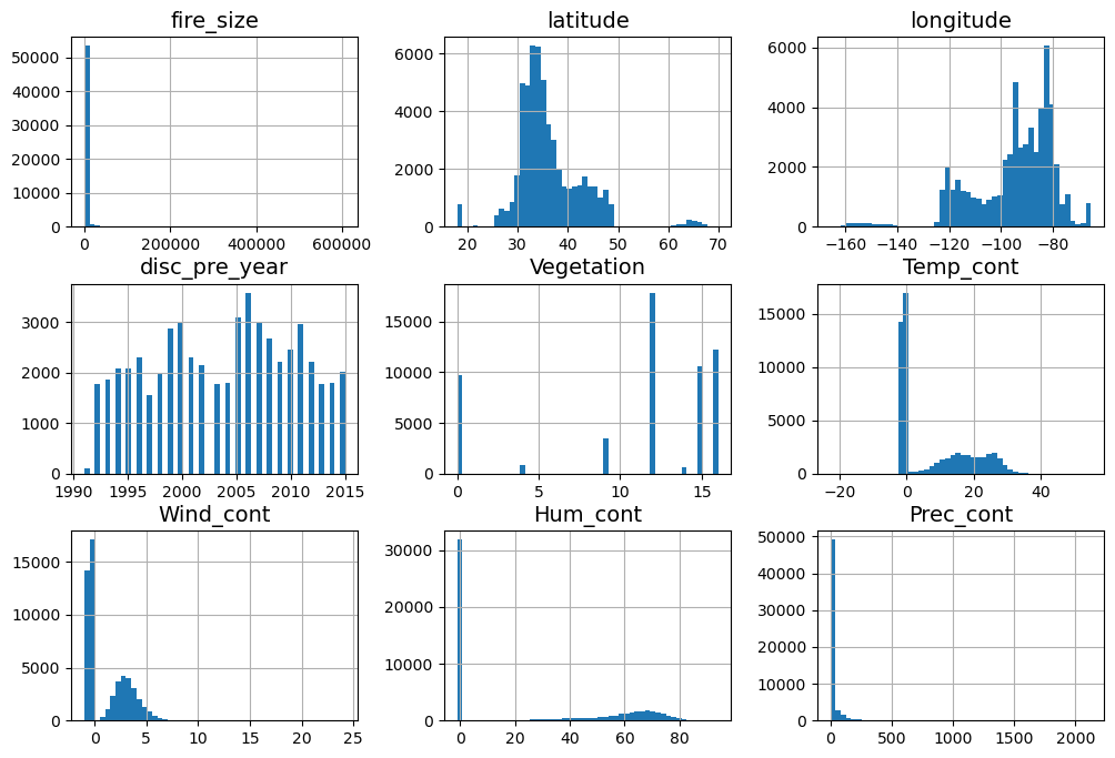
Explore the distributions of the variables in our data set#
Since we have 43 variables, we will focus on a subset of these variables for now. We want to understand how the variables are distributed. We’ll focus on the size of the fire, its location, how long it took to put out, the year it was discovered, the type of vegetation, and historical metereological variables (Temperature, Wind, Humidity, and Precipitation) averaged over the time it took to put out the fire.
variables = ["fire_size","fire_size_class","latitude","longitude","putout_time","disc_pre_year","Vegetation","Temp_cont","Wind_cont","Hum_cont","Prec_cont"]
First we will put this subsection of the data into a DataFrame object by using the variable names we have chosen.
df = wildfiresdb[variables].copy()
df.head()
| fire_size | fire_size_class | latitude | longitude | putout_time | disc_pre_year | Vegetation | Temp_cont | Wind_cont | Hum_cont | Prec_cont | |
|---|---|---|---|---|---|---|---|---|---|---|---|
| 0 | 10.0 | C | 18.105072 | -66.753044 | NaN | 2007 | 12 | 24.527961 | 3.250413 | 78.724370 | 0.0 |
| 1 | 3.0 | B | 35.038330 | -87.610000 | NaN | 2006 | 15 | 10.448298 | 2.122320 | 81.682678 | 86.8 |
| 2 | 60.0 | C | 34.947800 | -88.722500 | NaN | 2004 | 16 | 13.696600 | 3.369050 | 65.063800 | 124.5 |
| 3 | 1.0 | B | 39.641400 | -119.308300 | 0 days 00:00:00.000000000 | 2005 | 0 | 0.000000 | 0.000000 | 0.000000 | 0.0 |
| 4 | 2.0 | B | 30.700600 | -90.591400 | NaN | 1999 | 12 | -1.000000 | -1.000000 | -1.000000 | -1.0 |
You can explore the data in various ways.
First, how many samples are in our data set?
print("Number of rows: " + str(len(df)))
Number of rows: 55367
We can use matplotlib to visualize the marginal distributions of our variables using the hist function:
import matplotlib.pyplot as plt

# extra code – the next 5 lines define the default font sizes
plt.rc('font', size=14)
plt.rc('axes', labelsize=14, titlesize=14)
plt.rc('legend', fontsize=14)
plt.rc('xtick', labelsize=10)
plt.rc('ytick', labelsize=10)

df.hist(bins=50, figsize=(12, 8))
#save_fig("attribute_histogram_plots")  # extra code
plt.show()
Another useful python package that we can use is seaborn.
Warning! Seaborn can typically be quite slow, especially if you have a large data set or many variables. One simple way to deal with this is to randomly subsample the data, and visualize only a fraction of the data set.
import seaborn as sns
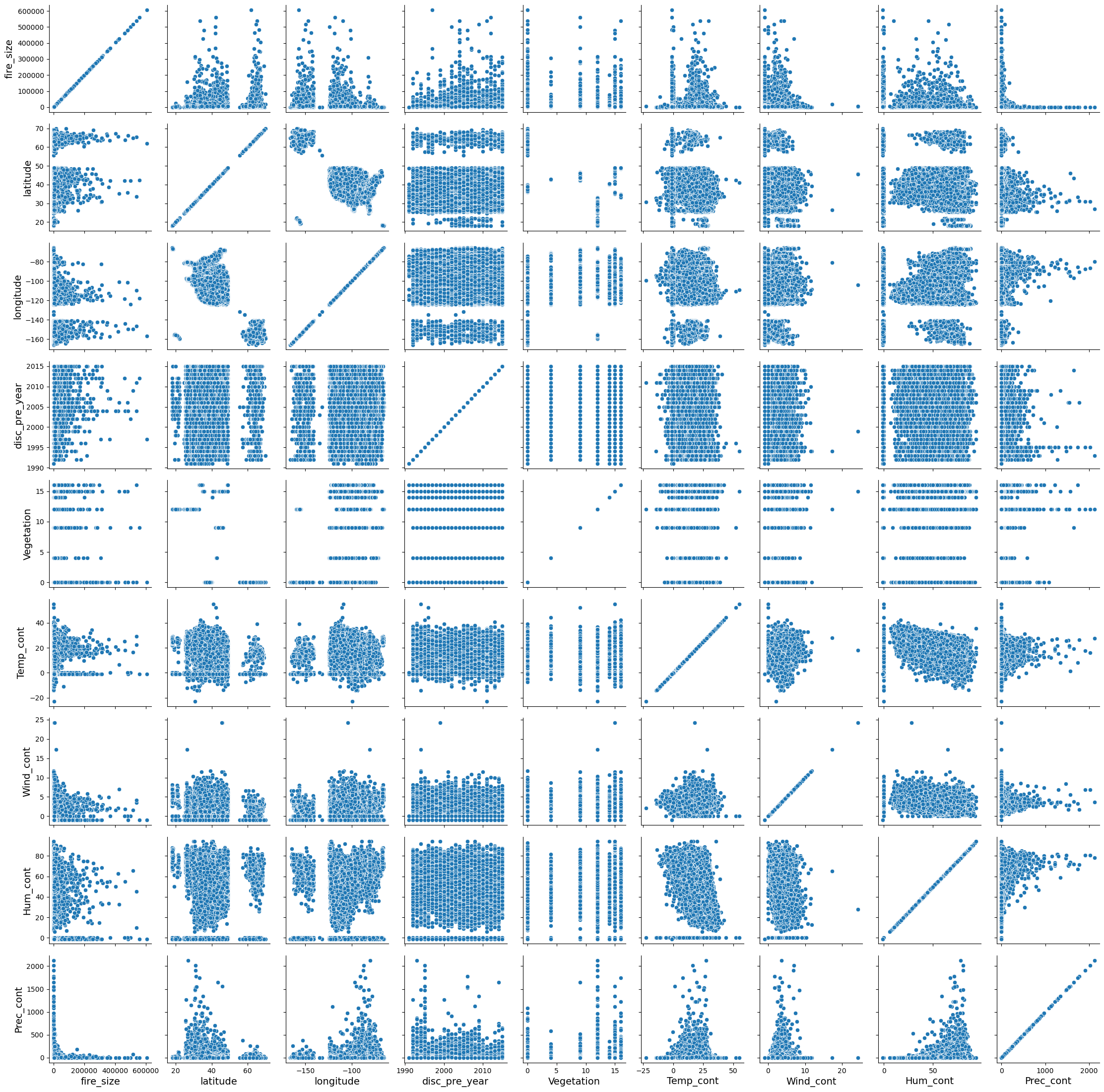
We can look at how the variables are correlated with one another using the PairGrid function
We need both of the lines below to create the plot. The first line just constructs a blank grid of subplots with each row and column corresponding to a numeric value in the data set. The second line draws a bivariate plot on every axis.
g = sns.PairGrid(df)
g.map(sns.scatterplot)
<seaborn.axisgrid.PairGrid at 0x1514523d0>
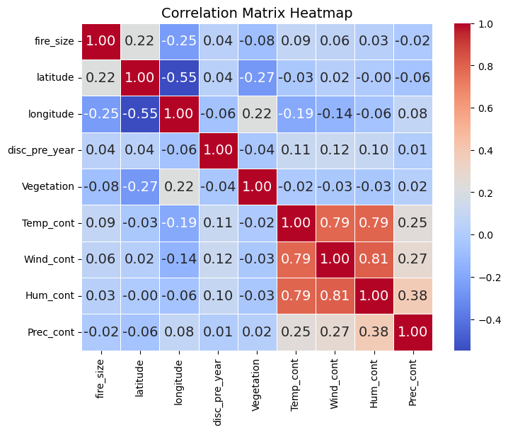
We can also look for correlations between the variables in our data set, using the pandas DataFrame corr method. The numeric_only argument needs to be set to True to avoid an error. This makes sure it only uses the variables in our dataframe that have numeric values.
corr_matrix = df.corr(numeric_only=True)
# Create a heatmap of the correlation matrix
plt.figure(figsize=(8, 6)) # Adjust figure size as needed
sns.heatmap(corr_matrix, annot=True, cmap='coolwarm', fmt=".2f", linewidths=.5)
plt.title('Correlation Matrix Heatmap')
plt.show()
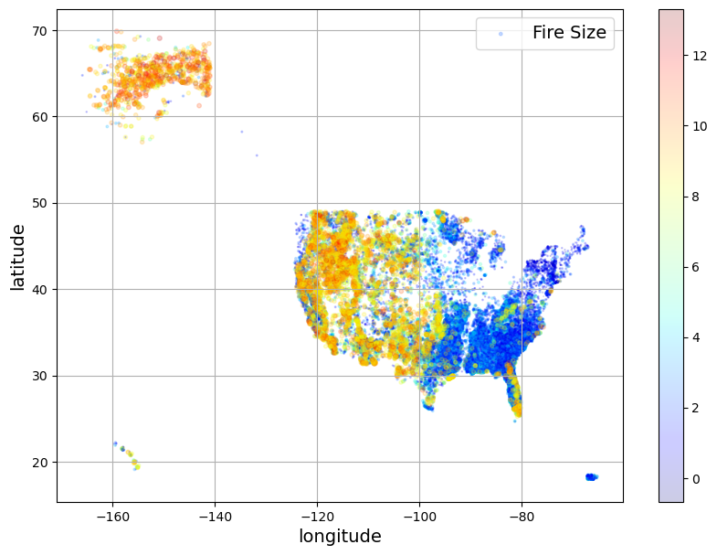
Visualize the data spatially#
Since we have latitude and longitude, we can also visualize the spatial distribution of the points in our data set. Looking at fire size, it’s clear that the largest fires occur for the most part in the Western US.
import numpy as np

df.plot(kind='scatter',x='longitude',y='latitude',grid=True,alpha=0.2,
                s = np.log(df["fire_size"]),label = "Fire Size",
                c = np.log(df["fire_size"]),cmap="jet",colorbar = True, legend = True, sharex=False,figsize=(10,7))
plt.show()
/opt/anaconda3/envs/ML4Climate2025/lib/python3.8/site-packages/matplotlib/collections.py:963: RuntimeWarning: invalid value encountered in sqrt
  scale = np.sqrt(self._sizes) * dpi / 72.0 * self._factor
Handling missing/irregular data#
The column putout_time contains many NaN values, because data on how long it took to put out the fire is not available for every fire.
First, we can try to understand why data might be missing.
no_putout_time = pd.isna(df['putout_time'])
Let’s compare the mean size of the fires which have no data for putout_time to the mean size of the fires which do have data:
print("Mean size of fires with NaN for putout_time:")
(df['fire_size'][no_putout_time]).mean()
Mean size of fires with NaN for putout_time:
415.81547412190747
print("Mean size of fires with values for putout_time:")
(df['fire_size'][~no_putout_time]).mean()
Mean size of fires with values for putout_time:
3818.859229537432
This suggests that smaller fires typically don’t have data about putout_time associated with them.
putout_time is currently formatted as string timestamps, rather than floating point numbers, and they are unfortunately not all in the same format. We can see this by printing out the unique values from this column.
unique = df['putout_time'].unique()
unique
array([nan, '0 days 00:00:00.000000000', '1 days 00:00:00.000000000',
       '2 days 00:00:00.000000000', '3 days 00:00:00.000000000',
       '26 days 00:00:00.000000000', '9 days 00:00:00.000000000',
       '4 days 00:00:00.000000000', '18 days 00:00:00.000000000',
       '5 days 00:00:00.000000000', '16 days 00:00:00.000000000',
       '7 days 00:00:00.000000000', '19 days 00:00:00.000000000',
       '12 days 00:00:00.000000000', '6 days 00:00:00.000000000',
       '167 days 00:00:00.000000000', '8 days 00:00:00.000000000',
       '69 days 00:00:00.000000000', '31 days 00:00:00.000000000',
       '36 days 00:00:00.000000000', '29 days 00:00:00.000000000',
       '15 days 00:00:00.000000000', '92 days 00:00:00.000000000',
       '91 days 00:00:00.000000000', '10 days 00:00:00.000000000',
       '11 days 00:00:00.000000000', '63 days 00:00:00.000000000',
       '118 days 00:00:00.000000000', '13 days 00:00:00.000000000',
       '59 days 00:00:00.000000000', '93 days 00:00:00.000000000',
       '28 days 00:00:00.000000000', '127 days 00:00:00.000000000',
       '50 days 00:00:00.000000000', '30 days 00:00:00.000000000',
       '152 days 00:00:00.000000000', '54 days 00:00:00.000000000',
       '25 days 00:00:00.000000000', '47 days 00:00:00.000000000',
       '55 days 00:00:00.000000000', '108 days 00:00:00.000000000',
       '39 days 00:00:00.000000000', '104 days 00:00:00.000000000',
       '17 days 00:00:00.000000000', '80 days 00:00:00.000000000',
       '22 days 00:00:00.000000000', '20 days 00:00:00.000000000',
       '97 days 00:00:00.000000000', '84 days 00:00:00.000000000',
       '81 days 00:00:00.000000000', '67 days 00:00:00.000000000',
       '14 days 00:00:00.000000000', '60 days 00:00:00.000000000',
       '62 days 00:00:00.000000000', '103 days 00:00:00.000000000',
       '24 days 00:00:00.000000000', '193 days 00:00:00.000000000',
       '117 days 00:00:00.000000000', '116 days 00:00:00.000000000',
       '41 days 00:00:00.000000000', '61 days 00:00:00.000000000',
       '145 days 00:00:00.000000000', '106 days 00:00:00.000000000',
       '94 days 00:00:00.000000000', '70 days 00:00:00.000000000',
       '43 days 00:00:00.000000000', '90 days 00:00:00.000000000',
       '35 days 00:00:00.000000000', '40 days 00:00:00.000000000',
       '21 days 00:00:00.000000000', '65 days 00:00:00.000000000',
       '23 days 00:00:00.000000000', '89 days 00:00:00.000000000',
       '114 days 00:00:00.000000000', '57 days 00:00:00.000000000',
       '27 days 00:00:00.000000000', '46 days 00:00:00.000000000',
       '87 days 00:00:00.000000000', '74 days 00:00:00.000000000',
       '37 days 00:00:00.000000000', '42 days 00:00:00.000000000',
       '73 days 00:00:00.000000000', '148 days 00:00:00.000000000',
       '141 days 00:00:00.000000000', '122 days 00:00:00.000000000',
       '66 days 00:00:00.000000000', '44 days 00:00:00.000000000',
       '88 days 00:00:00.000000000', '161 days 00:00:00.000000000',
       '34 days 00:00:00.000000000', '132 days 00:00:00.000000000',
       '140 days 00:00:00.000000000', '45 days 00:00:00.000000000',
       '102 days 00:00:00.000000000', '121 days 00:00:00.000000000',
       '51 days 00:00:00.000000000', '261 days 00:00:00.000000000',
       '77 days 00:00:00.000000000', '48 days 00:00:00.000000000',
       '53 days 00:00:00.000000000', '71 days 00:00:00.000000000',
       '56 days 00:00:00.000000000', '79 days 00:00:00.000000000',
       '85 days 00:00:00.000000000', '222 days 00:00:00.000000000',
       '76 days 00:00:00.000000000', '58 days 00:00:00.000000000',
       '72 days 00:00:00.000000000', '83 days 00:00:00.000000000',
       '32 days 00:00:00.000000000', '131 days 00:00:00.000000000',
       '52 days 00:00:00.000000000', '99 days 00:00:00.000000000',
       '112 days 00:00:00.000000000', '213 days 00:00:00.000000000',
       '135 days 00:00:00.000000000', '168 days 00:00:00.000000000',
       '68 days 00:00:00.000000000', '33 days 00:00:00.000000000',
       '101 days 00:00:00.000000000', '64 days 00:00:00.000000000',
       '38 days 00:00:00.000000000', '115 days 00:00:00.000000000',
       '165 days 00:00:00.000000000', '119 days 00:00:00.000000000',
       '146 days 00:00:00.000000000', '136 days 00:00:00.000000000',
       '110 days 00:00:00.000000000', '255 days 00:00:00.000000000',
       '86 days 00:00:00.000000000', '49 days 00:00:00.000000000',
       '184 days 00:00:00.000000000', '78 days 00:00:00.000000000',
       '96 days 00:00:00.000000000', '3287 days 00:00:00.000000000',
       '211 days 00:00:00.000000000', '178 days 00:00:00.000000000', '21',
       '11', '77', '75', '87', '67', '66', '22', '10', '2', '9', '1', '3',
       '6', '18', '12', '5', '13', '27', '8', '7', '4', '0', '82', '32',
       '80', '49', '60', '99', '91', '84', '78', '54', '71', '51', '30',
       '14', '94', '45', '42', '56', '58', '55', '33', '53', '17', '31',
       '23', '29', '50', '92', '79', '47', '20', '15', '115', '28', '46',
       '73', '72', '83', '90', '88', '89', '64', '81', '19', '37', '39',
       '43', '38', '101', '24', '112', '86', '74', '26', '110', '108',
       '35', '44', '36', '59', '68', '70', '96', '34', '48', '116', '63',
       '40', '98', '85', '16', '102', '131', '142', '128', '76', '25',
       '52', '93', '118', '107', '97', '104', '65', '129', '111', '106',
       '103', '114', '61', '62', '122', '121', '41', '144', '155', '117',
       '57', '105', '119', '113', '138', '100', '312', '125', '95', '132',
       '126', '164', '120', '163', '184', '177', '145', '134', '109',
       '127', '147', '124', '141', '139', '150', '123', '69', '137',
       '148', '136', '151', '140', '133', '146', '204', '178', '143',
       '237', '153', '371', '170'], dtype=object)
Since the information that we are interested in is the first “word” in each string, we can use the string split method to get the number of days it took to put out a fire, and put this into a new column in our data frame. We also want the variable to be a floating point number (not a string) so that we can use it in our (future) machine learning model.
df['putout_time_float'] = df['putout_time'].str.split().str[0].astype(float)
df['putout_time_float']
0         NaN
1         NaN
2         NaN
3         0.0
4         NaN
         ...
55362     NaN
55363    22.0
55364     NaN
55365    43.0
55366     NaN
Name: putout_time_float, Length: 55367, dtype: float64
df['putout_time_float'].describe()
count    27477.000000
mean         6.033592
std         27.803757
min          0.000000
25%          0.000000
50%          0.000000
75%          1.000000
max       3287.000000
Name: putout_time_float, dtype: float64
df
| fire_size | fire_size_class | latitude | longitude | putout_time | disc_pre_year | Vegetation | Temp_cont | Wind_cont | Hum_cont | Prec_cont | putout_time_float | |
|---|---|---|---|---|---|---|---|---|---|---|---|---|
| 0 | 10.0 | C | 18.105072 | -66.753044 | NaN | 2007 | 12 | 24.527961 | 3.250413 | 78.724370 | 0.0 | NaN |
| 1 | 3.0 | B | 35.038330 | -87.610000 | NaN | 2006 | 15 | 10.448298 | 2.122320 | 81.682678 | 86.8 | NaN |
| 2 | 60.0 | C | 34.947800 | -88.722500 | NaN | 2004 | 16 | 13.696600 | 3.369050 | 65.063800 | 124.5 | NaN |
| 3 | 1.0 | B | 39.641400 | -119.308300 | 0 days 00:00:00.000000000 | 2005 | 0 | 0.000000 | 0.000000 | 0.000000 | 0.0 | 0.0 |
| 4 | 2.0 | B | 30.700600 | -90.591400 | NaN | 1999 | 12 | -1.000000 | -1.000000 | -1.000000 | -1.0 | NaN |
| ... | ... | ... | ... | ... | ... | ... | ... | ... | ... | ... | ... | ... |
| 55362 | 6289.0 | G | 39.180000 | -96.784167 | NaN | 2015 | 0 | 13.242324 | 3.804803 | 55.042092 | 249.0 | NaN |
| 55363 | 70868.0 | G | 38.342719 | -120.695967 | 22 | 2015 | 0 | -1.000000 | -1.000000 | -1.000000 | -1.0 | 22.0 |
| 55364 | 5702.0 | G | 37.262607 | -119.511139 | NaN | 2015 | 0 | 27.646067 | 2.529158 | 35.924406 | 0.0 | NaN |
| 55365 | 3261.0 | F | 40.604300 | -123.080450 | 43 | 2015 | 15 | -1.000000 | -1.000000 | -1.000000 | -1.0 | 43.0 |
| 55366 | 76067.0 | G | 38.843988 | -122.759707 | NaN | 2015 | 0 | 19.016883 | 1.208073 | 58.063802 | 18.8 | NaN |
55367 rows × 12 columns
We’ll drop the original column now, since we have fixed the irregular data
df = df.drop(['putout_time'],axis=1)
df.head()
| fire_size | fire_size_class | latitude | longitude | disc_pre_year | Vegetation | Temp_cont | Wind_cont | Hum_cont | Prec_cont | putout_time_float | |
|---|---|---|---|---|---|---|---|---|---|---|---|
| 0 | 10.0 | C | 18.105072 | -66.753044 | 2007 | 12 | 24.527961 | 3.250413 | 78.724370 | 0.0 | NaN |
| 1 | 3.0 | B | 35.038330 | -87.610000 | 2006 | 15 | 10.448298 | 2.122320 | 81.682678 | 86.8 | NaN |
| 2 | 60.0 | C | 34.947800 | -88.722500 | 2004 | 16 | 13.696600 | 3.369050 | 65.063800 | 124.5 | NaN |
| 3 | 1.0 | B | 39.641400 | -119.308300 | 2005 | 0 | 0.000000 | 0.000000 | 0.000000 | 0.0 | 0.0 |
| 4 | 2.0 | B | 30.700600 | -90.591400 | 1999 | 12 | -1.000000 | -1.000000 | -1.000000 | -1.0 | NaN |
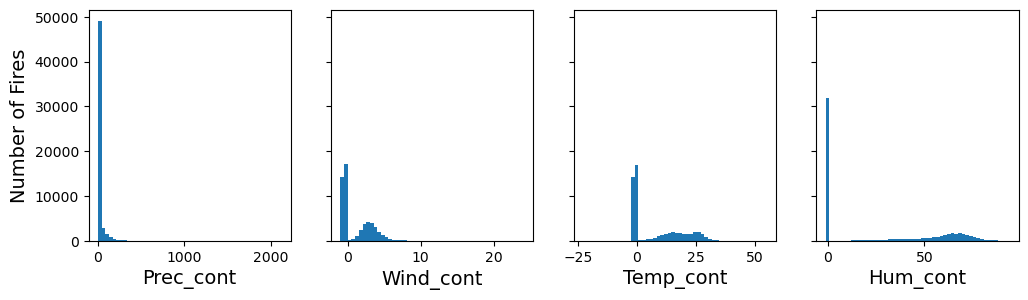
If we look at the meteorological variables (Prec_cont, Wind_cont, Temp_cont, Hum_cont), we also notice that the distributions look strange. This is because they have 0 and -1 for missing values. We can guess this because it’s not physically reasonable that these values are negative, or that the Wind_cont, Temp_cont, Hum_cont are exactly 0.0000, especially during fire season.
fig, axs = plt.subplots(1, 4, figsize=(12, 3), sharey=True)
axs[0].hist(df["Prec_cont"], bins=50)
axs[1].hist(df["Wind_cont"], bins=50)
axs[2].hist(df["Temp_cont"], bins=50)
axs[3].hist(df["Hum_cont"], bins=50)
axs[0].set_xlabel("Prec_cont")
axs[1].set_xlabel("Wind_cont")
axs[2].set_xlabel("Temp_cont")
axs[3].set_xlabel("Hum_cont")
axs[0].set_ylabel("Number of Fires")

plt.show()
df["Temp_cont"]
0        24.527961
1        10.448298
2        13.696600
3         0.000000
4        -1.000000
           ...
55362    13.242324
55363    -1.000000
55364    27.646067
55365    -1.000000
55366    19.016883
Name: Temp_cont, Length: 55367, dtype: float64
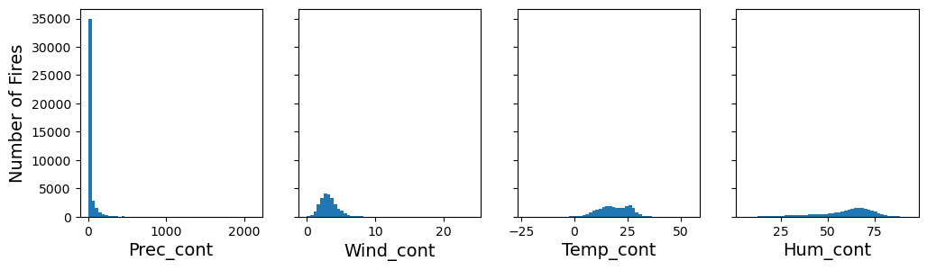
We can replace these suspicious values with NaN’s using the replace method.
df["Temp_cont"] = df["Temp_cont"].replace([0.0000,-1.0000], np.nan)
df["Hum_cont"] = df["Hum_cont"].replace([0.0000,-1.0000], np.nan)
df["Wind_cont"] = df["Wind_cont"].replace([0.0000,-1.0000], np.nan)
df["Prec_cont"] = df["Prec_cont"].replace([-1.0000], np.nan)
fig, axs = plt.subplots(1, 4, figsize=(12, 3), sharey=True)
axs[0].hist(df["Prec_cont"], bins=50)
axs[1].hist(df["Wind_cont"], bins=50)
axs[2].hist(df["Temp_cont"], bins=50)
axs[3].hist(df["Hum_cont"], bins=50)
axs[0].set_xlabel("Prec_cont")
axs[1].set_xlabel("Wind_cont")
axs[2].set_xlabel("Temp_cont")
axs[3].set_xlabel("Hum_cont")
axs[0].set_ylabel("Number of Fires")

plt.show()
Now that we have fixed the irregular data, we need to figure out what to do with the NaN values.
One very simple way to deal with these missing data is to just drop all of the rows where there are no values for putout_time, using the dropna() method:
df_cleaned = df.dropna().copy()
A disadvantage of dropping rows it that we end up with less data, so other approaches such as imputation can be preferable if our data set is small. After removing all of the bad rows, we are down to 10% of our original data set!
print("Number of rows (before removing NaN's): " + str(len(df)))
print("Number of rows (after removing NaN's): " + str(len(df_cleaned)))
Number of rows (before removing NaN's): 55367
Number of rows (after removing NaN's): 5892
We can also remove the very high outliers for putout_time_float (>99.995%):
q_hi  = df_cleaned['putout_time_float'].quantile(0.99995)
print(q_hi)

df_filtered = df_cleaned[(df_cleaned['putout_time_float'] < q_hi)].dropna().copy()
338.5995000000421
print("Number of rows (before removing outliers): " + str(len(df_cleaned)))
print("Number of rows (after removing outliers): " + str(len(df_filtered)))
Number of rows (before removing outliers): 5892
Number of rows (after removing outliers): 5891
We can also fill the NaN’s with a value instead, using the fillna() method:
df_filled = df.fillna(0).copy()
df_filled
| fire_size | fire_size_class | latitude | longitude | disc_pre_year | Vegetation | Temp_cont | Wind_cont | Hum_cont | Prec_cont | putout_time_float | |
|---|---|---|---|---|---|---|---|---|---|---|---|
| 0 | 10.0 | C | 18.105072 | -66.753044 | 2007 | 12 | 24.527961 | 3.250413 | 78.724370 | 0.0 | 0.0 |
| 1 | 3.0 | B | 35.038330 | -87.610000 | 2006 | 15 | 10.448298 | 2.122320 | 81.682678 | 86.8 | 0.0 |
| 2 | 60.0 | C | 34.947800 | -88.722500 | 2004 | 16 | 13.696600 | 3.369050 | 65.063800 | 124.5 | 0.0 |
| 3 | 1.0 | B | 39.641400 | -119.308300 | 2005 | 0 | 0.000000 | 0.000000 | 0.000000 | 0.0 | 0.0 |
| 4 | 2.0 | B | 30.700600 | -90.591400 | 1999 | 12 | 0.000000 | 0.000000 | 0.000000 | 0.0 | 0.0 |
| ... | ... | ... | ... | ... | ... | ... | ... | ... | ... | ... | ... |
| 55362 | 6289.0 | G | 39.180000 | -96.784167 | 2015 | 0 | 13.242324 | 3.804803 | 55.042092 | 249.0 | 0.0 |
| 55363 | 70868.0 | G | 38.342719 | -120.695967 | 2015 | 0 | 0.000000 | 0.000000 | 0.000000 | 0.0 | 22.0 |
| 55364 | 5702.0 | G | 37.262607 | -119.511139 | 2015 | 0 | 27.646067 | 2.529158 | 35.924406 | 0.0 | 0.0 |
| 55365 | 3261.0 | F | 40.604300 | -123.080450 | 2015 | 15 | 0.000000 | 0.000000 | 0.000000 | 0.0 | 43.0 |
| 55366 | 76067.0 | G | 38.843988 | -122.759707 | 2015 | 0 | 19.016883 | 1.208073 | 58.063802 | 18.8 | 0.0 |
55367 rows × 11 columns
Rather than filling with a specific value, it’s also possible to fill with the median or mean of the column.
df_fill_mean= df.copy()

meantime = df['putout_time_float'].mean()
df_fill_mean['putout_time_float'].fillna(meantime,inplace=True)
df_fill_mean
| fire_size | fire_size_class | latitude | longitude | disc_pre_year | Vegetation | Temp_cont | Wind_cont | Hum_cont | Prec_cont | putout_time_float | |
|---|---|---|---|---|---|---|---|---|---|---|---|
| 0 | 10.0 | C | 18.105072 | -66.753044 | 2007 | 12 | 24.527961 | 3.250413 | 78.724370 | 0.0 | 6.033592 |
| 1 | 3.0 | B | 35.038330 | -87.610000 | 2006 | 15 | 10.448298 | 2.122320 | 81.682678 | 86.8 | 6.033592 |
| 2 | 60.0 | C | 34.947800 | -88.722500 | 2004 | 16 | 13.696600 | 3.369050 | 65.063800 | 124.5 | 6.033592 |
| 3 | 1.0 | B | 39.641400 | -119.308300 | 2005 | 0 | NaN | NaN | NaN | 0.0 | 0.000000 |
| 4 | 2.0 | B | 30.700600 | -90.591400 | 1999 | 12 | NaN | NaN | NaN | NaN | 6.033592 |
| ... | ... | ... | ... | ... | ... | ... | ... | ... | ... | ... | ... |
| 55362 | 6289.0 | G | 39.180000 | -96.784167 | 2015 | 0 | 13.242324 | 3.804803 | 55.042092 | 249.0 | 6.033592 |
| 55363 | 70868.0 | G | 38.342719 | -120.695967 | 2015 | 0 | NaN | NaN | NaN | NaN | 22.000000 |
| 55364 | 5702.0 | G | 37.262607 | -119.511139 | 2015 | 0 | 27.646067 | 2.529158 | 35.924406 | 0.0 | 6.033592 |
| 55365 | 3261.0 | F | 40.604300 | -123.080450 | 2015 | 15 | NaN | NaN | NaN | NaN | 43.000000 |
| 55366 | 76067.0 | G | 38.843988 | -122.759707 | 2015 | 0 | 19.016883 | 1.208073 | 58.063802 | 18.8 | 6.033592 |
55367 rows × 11 columns
Finally, we can interpolate, using the interpolate() method. Interpolate refers to filling in using the values based on estimating from surrounding non-NaN data in a column.
df_interp = df.interpolate().copy()
Interpolation doesn’t make a lot of sense for this data set since the fires are independent of one another. Interpolation makes more sense in the context of a time series, where we are missing specific values in our sequence. To illustrate this, we will look at the effect of using the Interpolate() method on a sine wave that has 20% of its data missing.
This code just generates the time series and puts it into a dataframe
np.random.seed(42)
n = 100
t = np.linspace(0, 2 * np.pi, n)         # 0 → 2π
y = np.sin(t)
y_noisy = y+ np.random.normal(0, 0.1, n)

# knock out ~10 % of points
mask = np.random.choice(n, size=int(0.20 * n), replace=False)
y_noisy[mask] = np.nan

dfsine = pd.DataFrame({"t": t, "sine": y,"noisy_sine": y_noisy})
We can apply the interpolate function to the sine wave to estimate the missing values.
dfsine_interp = dfsine.interpolate().copy()
plt.scatter(dfsine['t'],dfsine['noisy_sine'],marker='o',facecolors='r',edgecolors='r',label="original")
plt.scatter(dfsine_interp['t'],dfsine_interp['noisy_sine'],marker='o',facecolors='none',edgecolors='k',label="interpolated")
plt.xlabel("t")
plt.ylabel("y")
plt.legend()
<matplotlib.legend.Legend at 0x157482640>
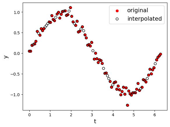
Using interpolation or filling missing values can potentially bias our data sets, so it’s important to keep in mind what problem we are interested in solving when choosing a method to deal with missing data.
Feature Scaling#
The sci-kit learn package has a number of built in functions for scaling variables.
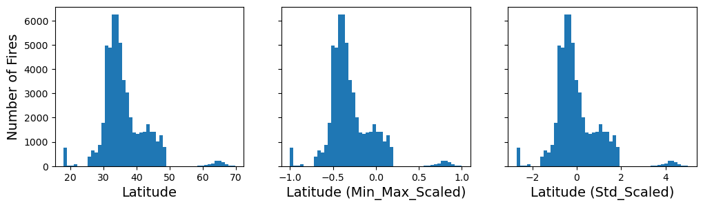
MinMaxScaler scales value between a minimum and maximum. We can set what range we want to end up with.
For a sample x, the MinMaxScaler is calculated as
X_std = (X - X.min(axis=0)) / (X.max(axis=0) - X.min(axis=0))
X_scaled = X_std * (max - min) + min
from sklearn.preprocessing import MinMaxScaler
min_max_scaler = MinMaxScaler(feature_range=(-1, 1))
latitude_min_max_scaled = min_max_scaler.fit_transform(df[["latitude"]])
The StandardScaler removes the mean and scales to unit variance. For a sample x, the standard scaler is calculated as
z = (x-u)/s
from sklearn.preprocessing import StandardScaler
std_scaler = StandardScaler()
latitude_std_scaled = std_scaler.fit_transform(df[["latitude"]])
fig, axs = plt.subplots(1, 3, figsize=(12, 3), sharey=True)
axs[0].hist(df["latitude"], bins=50)
axs[1].hist(latitude_min_max_scaled, bins=50)
axs[2].hist(latitude_std_scaled, bins=50)
axs[0].set_xlabel("Latitude")
axs[1].set_xlabel("Latitude (Min_Max_Scaled)")
axs[2].set_xlabel("Latitude (Std_Scaled)")
axs[0].set_ylabel("Number of Fires")

plt.show()
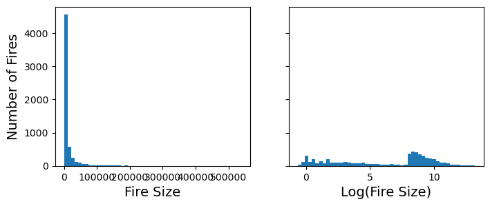
We can also do custom transformations using sci-kit learn’s FunctionTransformer method. For example, fire_size is not normally distributed, but rather strongly skewed towards smaller fires. We can log scale this variable using the FunctionTransformer
from sklearn.preprocessing import FunctionTransformer

log_transformer = FunctionTransformer(np.log, inverse_func=np.exp)
log_fire_size = log_transformer.transform(df_filtered[["fire_size"]])
fig, axs = plt.subplots(1, 2, figsize=(8, 3), sharey=True)
axs[0].hist(df_filtered["fire_size"], bins=50)
axs[1].hist(log_fire_size, bins=50)
axs[0].set_xlabel("Fire Size")
axs[1].set_xlabel("Log(Fire Size)")
axs[0].set_ylabel("Number of Fires")

plt.show()
df_filtered["log_fire_size"] = log_fire_size
Encoding categorical variables#
The fire_size_class is a categorical variable (it is a letter between A - G).
fire_size_class = df[["fire_size_class"]]
fire_size_class.head(8)
| fire_size_class | |
|---|---|
| 0 | C |
| 1 | B |
| 2 | C |
| 3 | B |
| 4 | B |
| 5 | B |
| 6 | B |
| 7 | B |
We can also check if our data set is balanced or not, by printing out the number of samples of each class in our data set.
fire_size_class_counts = df["fire_size_class"].value_counts()
print(fire_size_class_counts)
fire_size_class
B    36522
C    10811
G     3972
F     1968
D     1394
E      700
Name: count, dtype: int64
There are several different ways that we can encode this categorical variable for machine learning models. One is using the OrdinalEncoder function from sci-kit learn. This function will transform categories (B,C,D,E,…) to an integer label (0,1,2,3,…).
We will end up with a single column per original feature (or variable) in our data set.
OrdinalEncoder can be useful if our categories have a particular ordering to them (like fire size class does). However, it might not be a good choice for a feature like the state in which a fire occured, since we don’t have a particular ordering to the values in our data set in that case.
from sklearn.preprocessing import OrdinalEncoder

ordinal_encoder = OrdinalEncoder()
fire_size_class_encoded = ordinal_encoder.fit_transform(fire_size_class)
fire_size_class
| fire_size_class | |
|---|---|
| 0 | C |
| 1 | B |
| 2 | C |
| 3 | B |
| 4 | B |
| ... | ... |
| 55362 | G |
| 55363 | G |
| 55364 | G |
| 55365 | F |
| 55366 | G |
55367 rows × 1 columns
fire_size_class_encoded[:8]
array([[1.],
       [0.],
       [1.],
       [0.],
       [0.],
       [0.],
       [0.],
       [0.]])
ordinal_encoder.categories_
[array(['B', 'C', 'D', 'E', 'F', 'G'], dtype=object)]
An alternative way that we can encode a categorical variable is using the OneHotEncoder function from sci-kit learn. This function converts each category into a separate binary column. For example, a sample that is class B, would be one hot encoded as
[1, 0, 0, 0, 0, 0]
or for a sample that is a fire of class E, it would be encoded as
[0, 0, 0, 1, 0, 0]
We will end up with as many columns as we have classes in our data set. For the fire_size_class variable, this would add 6 columns, since there are 6 possible classes represented in our data set.
This is best to use when our categorical variables are nominal (unordered), and is best for many of the types of models that assume inputs are numerical and unstructured (linear models, neural networks), which we will discuss later in the course.
from sklearn.preprocessing import OneHotEncoder

cat_encoder = OneHotEncoder()
fire_size_class_hot = cat_encoder.fit_transform(fire_size_class)
fire_size_class_hot
<55367x6 sparse matrix of type '<class 'numpy.float64'>'
	with 55367 stored elements in Compressed Sparse Row format>
fire_size_class_hot.toarray()
array([[0., 1., 0., 0., 0., 0.],
       [1., 0., 0., 0., 0., 0.],
       [0., 1., 0., 0., 0., 0.],
       ...,
       [0., 0., 0., 0., 0., 1.],
       [0., 0., 0., 0., 1., 0.],
       [0., 0., 0., 0., 0., 1.]])
cat_encoder.categories_
[array(['B', 'C', 'D', 'E', 'F', 'G'], dtype=object)]
Creating a pipeline to preprocess our features#
df_filtered
| fire_size | fire_size_class | latitude | longitude | disc_pre_year | Vegetation | Temp_cont | Wind_cont | Hum_cont | Prec_cont | putout_time_float | log_fire_size | |
|---|---|---|---|---|---|---|---|---|---|---|---|---|
| 36 | 1420.0 | F | 33.241800 | -104.912200 | 1994 | 16 | 36.241176 | 4.217647 | 17.058824 | 0.0 | 1.0 | 7.258412 |
| 56 | 15.3 | C | 36.586500 | -96.323220 | 2015 | 0 | 5.258333 | 3.558333 | 71.500000 | 0.0 | 1.0 | 2.727853 |
| 57 | 270.0 | D | 35.473333 | -84.450000 | 1999 | 15 | 16.431034 | 0.982759 | 67.050000 | 0.0 | 1.0 | 5.598422 |
| 59 | 57.0 | C | 36.816667 | -82.651667 | 1995 | 0 | 13.002083 | 1.950000 | 37.854167 | 0.0 | 2.0 | 4.043051 |
| 78 | 450.0 | E | 34.330000 | -117.513056 | 2006 | 16 | 33.900000 | 2.237500 | 39.375000 | 0.0 | 1.0 | 6.109248 |
| ... | ... | ... | ... | ... | ... | ... | ... | ... | ... | ... | ... | ... |
| 55347 | 3200.0 | F | 46.679234 | -93.270841 | 2015 | 15 | 10.666667 | 4.813889 | 51.583333 | 0.0 | 1.0 | 8.070906 |
| 55349 | 17831.0 | G | 30.005000 | -100.391167 | 2015 | 12 | 28.250580 | 2.360093 | 58.243619 | 0.0 | 6.0 | 9.788694 |
| 55350 | 3452.0 | F | 30.400883 | -101.331933 | 2015 | 12 | 28.793750 | 3.082979 | 39.510638 | 0.0 | 2.0 | 8.146709 |
| 55351 | 8300.0 | G | 45.922100 | -111.422500 | 2015 | 15 | 11.032231 | 3.367769 | 48.628099 | 0.0 | 5.0 | 9.024011 |
| 55352 | 4704.0 | F | 48.937900 | -119.309100 | 2015 | 15 | 21.204970 | 4.537914 | 36.257773 | 4.4 | 140.0 | 8.456168 |
5891 rows × 12 columns
Let’s say that we are interested in predicting the time it takes to put out a fire, given the other variables in our data set. First, we will scale the putout_time_float using the standard scaler and put it into an array called y, since its our target variable.
std_scaler = StandardScaler()
y = std_scaler.fit_transform(df_filtered[["putout_time_float"]])
Next we will create a feature matrix X, which will be the input to our model. First let’s remove our target variable from the dataframe.
features = df_filtered.copy()
features = df_filtered.drop(["putout_time_float"],axis=1)
features
| fire_size | fire_size_class | latitude | longitude | disc_pre_year | Vegetation | Temp_cont | Wind_cont | Hum_cont | Prec_cont | log_fire_size | |
|---|---|---|---|---|---|---|---|---|---|---|---|
| 36 | 1420.0 | F | 33.241800 | -104.912200 | 1994 | 16 | 36.241176 | 4.217647 | 17.058824 | 0.0 | 7.258412 |
| 56 | 15.3 | C | 36.586500 | -96.323220 | 2015 | 0 | 5.258333 | 3.558333 | 71.500000 | 0.0 | 2.727853 |
| 57 | 270.0 | D | 35.473333 | -84.450000 | 1999 | 15 | 16.431034 | 0.982759 | 67.050000 | 0.0 | 5.598422 |
| 59 | 57.0 | C | 36.816667 | -82.651667 | 1995 | 0 | 13.002083 | 1.950000 | 37.854167 | 0.0 | 4.043051 |
| 78 | 450.0 | E | 34.330000 | -117.513056 | 2006 | 16 | 33.900000 | 2.237500 | 39.375000 | 0.0 | 6.109248 |
| ... | ... | ... | ... | ... | ... | ... | ... | ... | ... | ... | ... |
| 55347 | 3200.0 | F | 46.679234 | -93.270841 | 2015 | 15 | 10.666667 | 4.813889 | 51.583333 | 0.0 | 8.070906 |
| 55349 | 17831.0 | G | 30.005000 | -100.391167 | 2015 | 12 | 28.250580 | 2.360093 | 58.243619 | 0.0 | 9.788694 |
| 55350 | 3452.0 | F | 30.400883 | -101.331933 | 2015 | 12 | 28.793750 | 3.082979 | 39.510638 | 0.0 | 8.146709 |
| 55351 | 8300.0 | G | 45.922100 | -111.422500 | 2015 | 15 | 11.032231 | 3.367769 | 48.628099 | 0.0 | 9.024011 |
| 55352 | 4704.0 | F | 48.937900 | -119.309100 | 2015 | 15 | 21.204970 | 4.537914 | 36.257773 | 4.4 | 8.456168 |
5891 rows × 11 columns
Now we can apply a pipeline of transformations to our data set. sci-kit learn allows up to create separate pipelines for categorical and numerical variables and then run them on our entire dataframe simultaneously.
from sklearn.pipeline import make_pipeline
from sklearn.compose import ColumnTransformer
We need to separate our variables based on how we want to transform them though.
categorical_cols = ["fire_size_class"]
numerical_cols = ["fire_size","latitude","longitude","disc_pre_year","Vegetation","Temp_cont","Wind_cont","Hum_cont","Prec_cont","log_fire_size"]
cat_pipeline = make_pipeline(OrdinalEncoder(),StandardScaler())
num_pipeline = make_pipeline(MinMaxScaler())
preprocessor = ColumnTransformer([
    ("num",num_pipeline,numerical_cols),
    ("cat",cat_pipeline,categorical_cols)])
X = preprocessor.fit_transform(features)
X.shape
(5891, 11)
preprocessor.get_feature_names_out()
array(['num__fire_size', 'num__latitude', 'num__longitude',
       'num__disc_pre_year', 'num__Vegetation', 'num__Temp_cont',
       'num__Wind_cont', 'num__Hum_cont', 'num__Prec_cont',
       'num__log_fire_size', 'cat__fire_size_class'], dtype=object)
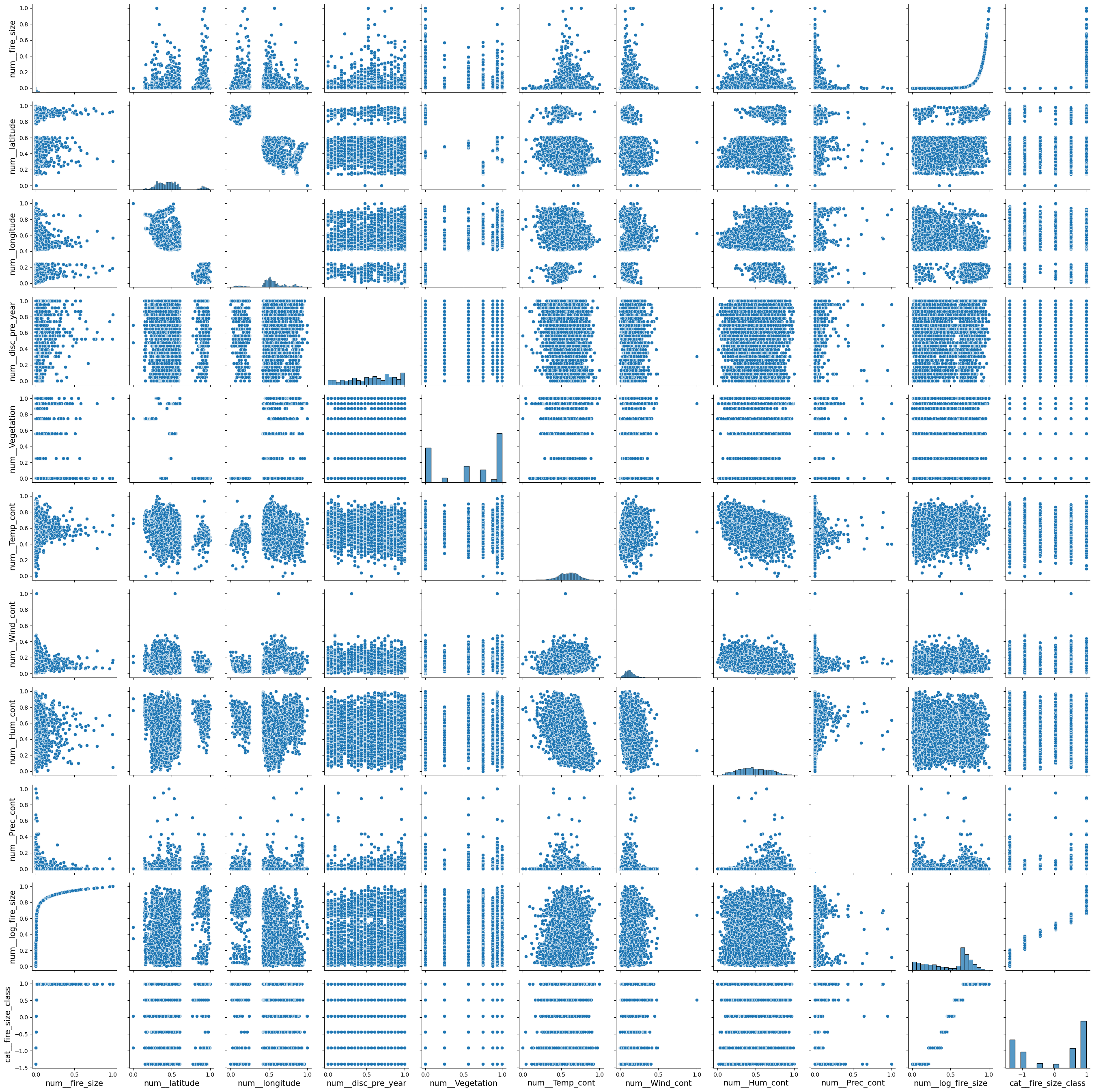
g = sns.PairGrid(pd.DataFrame(X,columns = preprocessor.get_feature_names_out()))
g.map_diag(sns.histplot)
g.map_offdiag(sns.scatterplot)
<seaborn.axisgrid.PairGrid at 0x161139880>
Creating a training, validation, and test data set#
Sci-kit learn has several built in functions to facilitate create separate training and test data sets. The simplest one to use is train_test_split, which returns the features and targets split into train and test data sets. If we want to also create a validation data set using this function, we will need to split the data set twice.
from sklearn.model_selection import train_test_split
X_train, X_test_val, y_train, y_test_val = train_test_split(X,y,test_size=0.5, random_state=42)
X_val, X_test, y_val, y_test = train_test_split(X_test_val,y_test_val,test_size=0.5, random_state=42)
print(X_train.shape,X_val.shape,X_test.shape)
(2945, 11) (1473, 11) (1473, 11)